- Part 1: Song length distributions with joy plots!
- Part 2: Breaking down the lyrics, word-by-word with tidytext
In Part 3 we get into the core element of our analysis, investigating the various sentiments and emotions expressed in Thrice’s lyrics!
Using the three sentiment lexicons included with the tidytext package, NRC, Bing, and AFINN we can categorize our tokenized lyrics data set and then perform a variety of transformations and manipulations to create some visualizations!
library(tidyverse)   # tidyr, dplyr, ggplot2

library(tidytext)
library(stringr)

library(scales)

library(wordcloud)
library(reshape2)
Let’s get started! Using the wordToken2 data set that we created in Part 2 we will filter out any numbers in our data set and then use a left_join() function to:
- grab a specific sentiment lexicon with the
get_sentiments()function - “join” the sentiment lexicon to the tokenized data set, specify
by = "word"
tidy_lyrics <- wordToken2 %>%
  select(-writers, -length, -lengthS)

emotions_lyrics_bing <- tidy_lyrics %>%
  filter(!grepl('[0-9]', word)) %>%
  left_join(get_sentiments("bing"), by = "word") %>%
  group_by(album) %>%
  mutate(sentiment = ifelse(is.na(sentiment), 'neutral', sentiment)) %>%   # add in neutral
  ungroup()

emotions_lyrics_bing %>%
  count(sentiment)
## # A tibble: 3 x 2
##   sentiment     n
##       <chr> <int>
## 1  negative   912
## 2   neutral  5095
## 3  positive   423
Unfortunately, the Bing lexicon counts most of the words in Thrice’s lyrics as neutral (transformed from NA) as not all words in our lyrics have a corresponding sentiment category in the lexicon.
We’ll come back to a more in-depth analysis of the nuances of each of the lexicons in the tidytext package a little bit later.
Most common positive and negative words in Thrice lyrics!
To have words with negative sentiment to have negative numbers we can create an if else statement that assigns -n to a word with a negative sentiment and to all else assign the regular n count. We’ll then order the words in these groups by the number of times they appear in the plot.
word_count <- emotions_lyrics_bing %>%
  count(word, sentiment, sort = T) %>%
  ungroup()

top_sentiments_bing <-  word_count %>%
  filter(sentiment != 'neutral') %>%
  group_by(sentiment) %>%
  top_n(5, n) %>%
  mutate(num = ifelse(sentiment == "negative", -n, n)) %>%
  select(-n) %>%
  mutate(word = reorder(word, num)) %>%
  ungroup()

ggplot(top_sentiments_bing, aes(reorder(word, num), num, fill = sentiment)) +
  geom_bar(stat = 'identity', alpha = 0.75) +
  scale_fill_manual(guide = F, values = c("black", "darkgreen")) +
  scale_y_continuous(limits = c(-40, 70), breaks = pretty_breaks(7)) +
  labs(x = '', y = "Number of Occurrences",
       title = 'Lyrics Sentiment of Thrice',
       subtitle = 'Most Common Positive and Negative Words') +
  theme_bw() +
  theme(axis.text.x = element_text(angle = 45, hjust = 1, size = 14, face = "bold"),
        panel.grid.minor = element_blank(),
        panel.grid.major.x = element_blank(),
        panel.grid.major.y = element_line(size = 1.1))
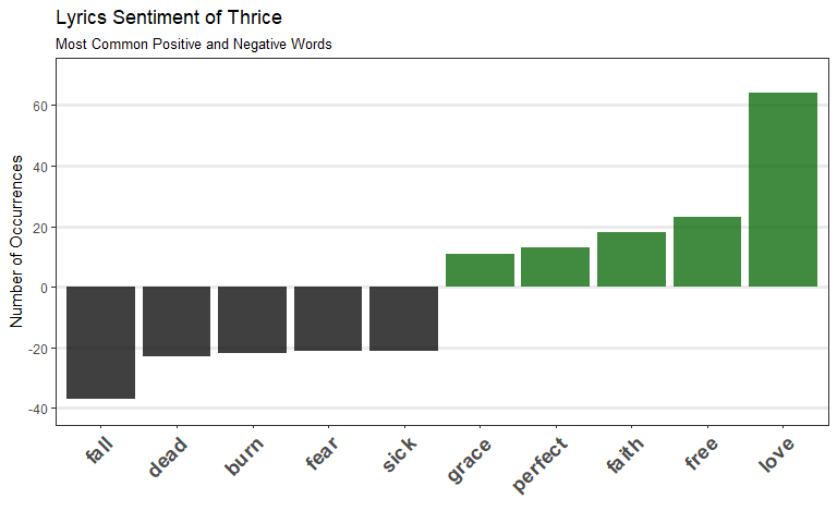
Reminiscent of the most common words plot (without “stop words”) from Part 2 except this time we’ve differentiated between words with positive sentiment and negative sentiment! Another way to visualize this is using a word cloud!
Word Cloud: Most Common Positive and Negative Words in Thrice Lyrics
library(wordcloud)   # to create wordcloud
library(reshape2)    # for acast() function

emotions_lyrics_bing %>%
  filter(sentiment != 'neutral') %>%
  count(word, sentiment, sort = T) %>%
  acast(word ~ sentiment, value.var = "n", fill = 0) %>%
  comparison.cloud(colors = c("black", "darkgreen"), title.size = 1.5)

# EDIT: with tidyverse, spread() instead of acast()
emotions_lyrics_bing %>%
  filter(sentiment != "neutral") %>%
  count(word, sentiment, sort = TRUE) %>%
  spread(sentiment, n, fill = 0L) %>%
  as.data.frame() %>%
  remove_rownames() %>%
  column_to_rownames("word") %>%
  comparison.cloud(colors = c("black", "darkgreen"), title.size = 1.5)
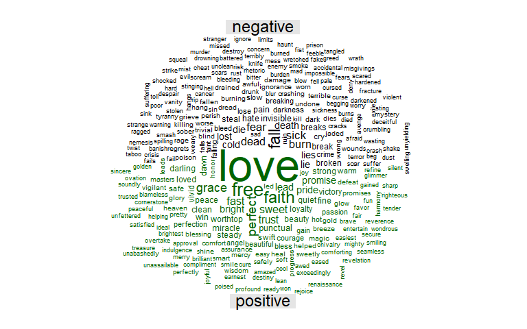 With the size of the word dictated by the size and central position in the cloud, this is another cool way to visualize the most common words. As seen before for positive words, Love appears the most whereas for negative, Fall appears most frequently.
Proportions of Positive and Negative Words
OK, now that we’ve looked at the most common words for either positive or negative sentiment, what proportion of these sentiments are present in within the entire lyrical data set? For this we can create
After filtering out the words categorized as neutral, we calculate the frequency by first grouping them along sentiment (the column specifying all the different emotion terms) and then counting the rows for each of these groups. Finally, we can calculate the percentage by dividing by the sum of all the rows in the data set.
pos_neg_bing <- tidy_lyrics %>%
  filter(!grepl('[0-9]', word)) %>%
  left_join(get_sentiments("bing"), by = "word") %>%
  mutate(sentiment = ifelse(is.na(sentiment), 'neutral', sentiment)) %>%
  group_by(album, sentiment) %>%
  summarize(n = n()) %>%
  mutate(percent = n / sum(n)) %>%
  select(-n) %>%
  ungroup()

pos_neg_bing %>%
  filter(sentiment != "neutral") %>%
  ggplot(aes(x = album, y = percent, color = sentiment, group = sentiment)) +
  geom_line(size = 1) +
  geom_point(size = 3) +
  scale_y_continuous(breaks = pretty_breaks(5), labels = percent_format()) +
  labs(x = "Album", y = "Emotion Words Count (as %)") +
  scale_color_manual(values = c(positive = "darkgreen", negative = "black")) +
  ggtitle("Proportion of Positive and Negative Words", subtitle = "Bing lexicon") +
  theme_bw() +
  theme(axis.text.x = element_text(angle = 45, hjust = 1, size = 11, face = "bold"),
        axis.title.x = element_blank(),
        axis.text.y = element_text(size = 11, face = "bold"))
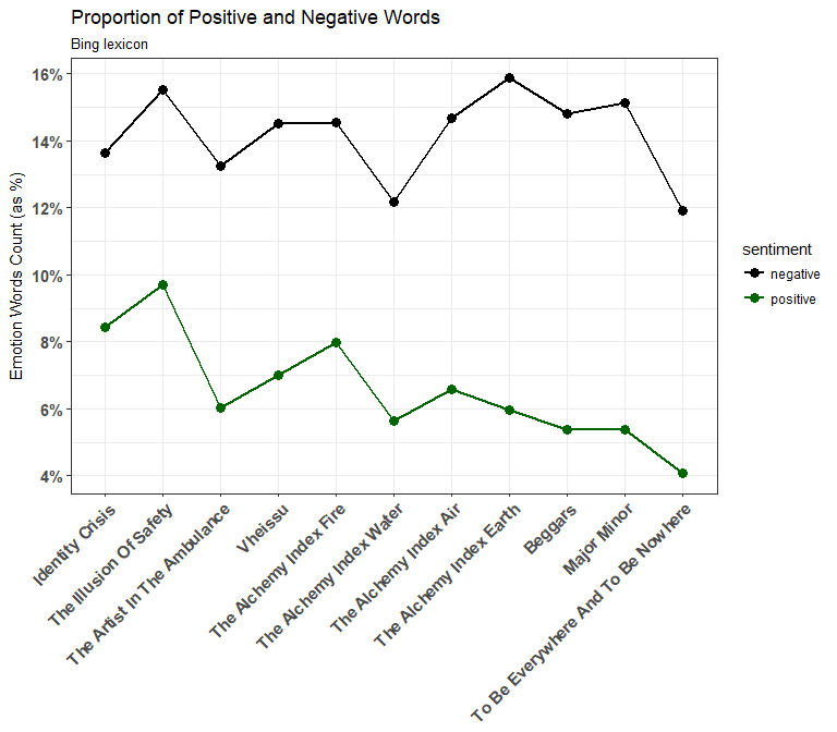
As we saw when we counted the words categorized for each sentiment at the beginning of the article, the neutral sentiment (not shown above) dominates, so both the positive and negative percentages move around a very low range. However, just looking at positive and negative sentiment groups may not be informative enough, let’s use the NRC lexicon to dig deeper!
Boxplot of emotion terms
The NRC lexicon not only categorizes words into positive and negative categories but also into eight different emotion terms, Anger, Anticipation, Disgust, Fear, Joy, Sadness, Surprise, and Trust.
After filtering out the words categorized as positive/negative as we are only comparing between the emotion terms here, and do the same calculations as we did for the previous plot.
Let’s use the colors from “Set1” in the RColorBrewer palettes to differentiate our emotion terms in the plot. We’ll use these assigned colors for some line charts later on too!
cols <- colorRampPalette(brewer.pal(n = 8, name = "Set1"))(8)

cols
## [1] "#E41A1C" "#377EB8" "#4DAF4A" "#984EA3" "#FF7F00" "#FFFF33" "#A65628"
## [8] "#F781BF"
”#E41A1C”, ”#377EB8”, etc. are the color hex codes for the colors in “Set1”. Now that we’ve extracted these color codes, let’s assign them to the emotion categories and then specify those are the colors we want to use for our lines with scale_color_manual() function.
cols <- c("anger" = "#E41A1C", "sadness" = "#377EB8", "disgust" = "#4DAF4A",
          "fear" = "#984EA3", "surprise" = "#FF7F00", "joy" = "#FFFF33",
          "anticipation" = "#A65628", "trust" = "#F781BF")

emotions_lyrics_nrc <- tidy_lyrics %>%
  left_join(get_sentiments("nrc"), by = "word") %>%
  filter(!(sentiment == "negative" | sentiment == "positive")) %>%
  mutate(sentiment = as.factor(sentiment)) %>%
  group_by(album, sentiment) %>%
  summarize(n = n()) %>%
  mutate(percent = n / sum(n)) %>%
  select(-n) %>%
  ungroup()

library(hrbrthemes)

emotions_lyrics_nrc %>%
  ggplot() +
  geom_boxplot(aes(x = reorder(sentiment, percent), y = percent, fill = sentiment)) +
  scale_y_continuous(breaks = pretty_breaks(5), labels = percent_format()) +
  scale_fill_manual(values = cols) +
  ggtitle("Distribution of Emotion Terms", subtitle = "n = 11 (Albums)") +
  labs(x = "Emotion Term", y = "Percentage") +
  theme_bw() +
  theme(legend.position = "none",
        axis.text.x = element_text(size = 11, face = "bold"),
        axis.text.y = element_text(size = 11, face = "bold"))
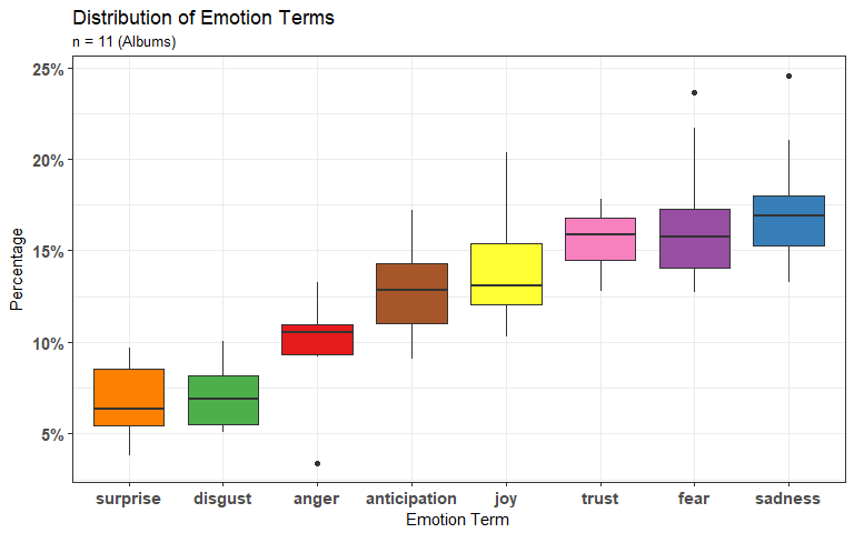
we can clearly see the box-plot distributions of the different emotion categories! As in any box plot, the black bar inside the box signifies the median, the hinges represent the 25th and 75th percentiles, while the whiskers extend to the value of 1.5 * IQR of their respective hinges, and the black dots are the outliers. But suppose we want to see how the lyrics change sentiment over time? We can create a bump chart that plots the different sentiment groups for each album in order of release-date!
emotions_lyrics_nrc %>%
  ggplot(aes(album, percent, color = sentiment, group = sentiment)) +
  geom_line(size = 1.5) +
  geom_point(size = 3.5) +
  scale_y_continuous(breaks = pretty_breaks(5), labels = percent_format()) +
  xlab("Album") + ylab("Proportion of Emotion Words") +
  ggtitle("Lyric Sentiments along Albums", subtitle = "From 2000-2016") +
  theme_bw() +
  theme(axis.text.x = element_text(angle = 45, hjust = 1, size = 11, face = "bold"),
        axis.title.x = element_blank(),
        axis.text.y = element_text(size = 11, face = "bold")) +
  scale_color_brewer(palette = "Set1")
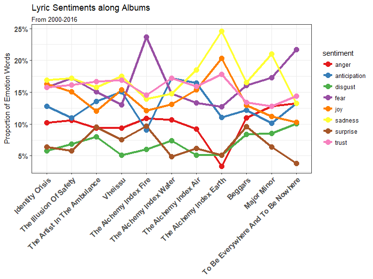
With EIGHT different emotions (Anger, Anticipation, Disgust, Fear, Joy, Sadness, Surprise, and Trust) in the NRC lexicon our nice graph looks quite cluttered and its hard to spot the trends, although it is quite clear that The Alchemy Index: Earth is the source of a lot of sudden increases/decreases in emotions.
To solve our current problem, let’s split the emotions into groups to be able to see changes better! These emotion terms won’t perfectly group up but let’s divide them into:
Anger,Disgust,Fear, andSadnessSurprise,Anticipation,Joy, andTrust
emotions_lyrics_nrc %>%
  filter(sentiment != "anger" & sentiment != "disgust" &
         sentiment != "fear" & sentiment != "sadness") %>%
  ggplot(aes(album, percent, color = sentiment, group = sentiment)) +
  geom_line(size = 1.5) +
  geom_point(size = 3.5) +
  scale_y_continuous(breaks = pretty_breaks(5), labels = percent_format()) +
  xlab("Album") + ylab("Proportion of Emotion Words") +
  ggtitle("Lyric Sentiments: Positive Emotion Terms", subtitle = "Release-date order (2000-2016)") +
  theme_bw() +
  theme(axis.text.x = element_text(angle = 45, hjust = 1, size = 11, face = "bold"),
        axis.title.x = element_blank(),
        axis.text.y = element_text(size = 11, face = "bold")) +
  scale_color_manual(values = cols, name = "Emotion Terms")
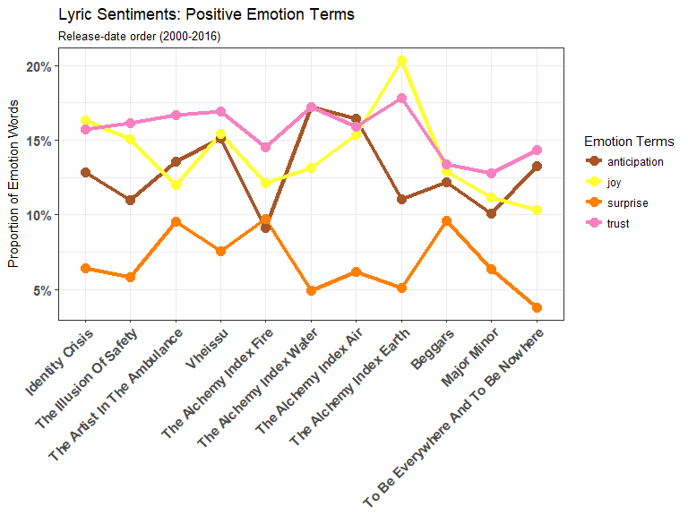
Anticipation seems to have dramatic dips in AI: Fire and AI: Earth compared to the preceding albums. Meanwhile Joy reaches the highest point for positive emotions at ~20% in AI: Earth while Trust seems to hover around 15-17% throughout Thrice’s discography until the last few albums.
And next, the negative emotions.
emotions_lyrics_nrc %>%
  filter(sentiment != "anticipation" & sentiment != "joy" &
         sentiment != "trust" & sentiment != "surprise") %>%
  ggplot(aes(album, percent, color = sentiment, group = sentiment)) +
  geom_line(size = 1.5) +
  geom_point(size = 3.5) +
  scale_y_continuous(breaks = pretty_breaks(5), labels = percent_format()) +
  labs(x = "Album", y = "Proportion of Emotion Words") +
  ggtitle("Lyric Sentiments: Negative Emotion Terms", subtitle = "Release-date order (2000-2016)") +
  theme_bw() +
  theme(axis.text.x = element_text(angle = 45, hjust = 1, size = 11, face = "bold"),
        axis.title.x = element_blank(),
        axis.text.y = element_text(size = 11, face = "bold")) +
  scale_color_manual(values = cols, name = "Emotion Terms")
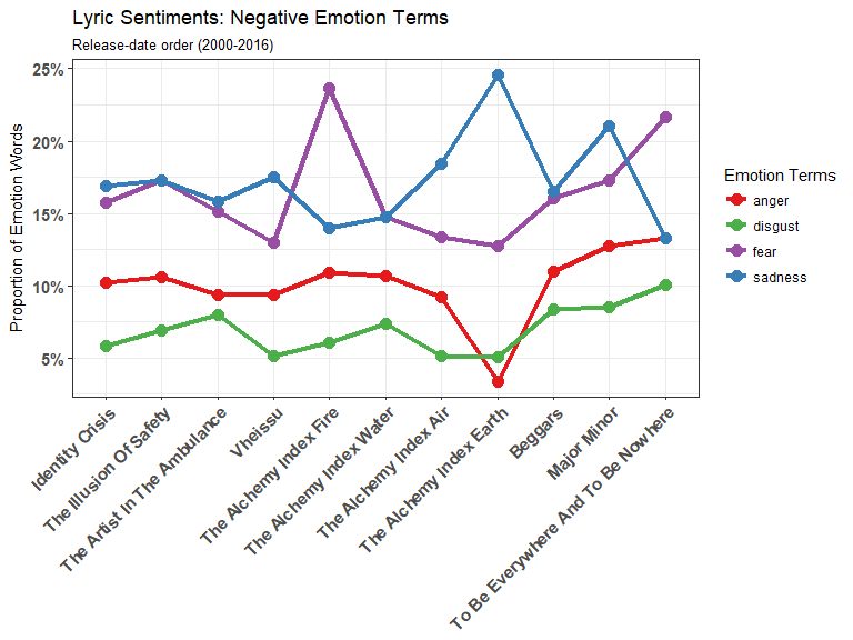
We can see that both Fear and Sadness have sudden spikes in AI:Fire and AI:Earth, which shows that there is a clear shift in emotional tone. Again, a caveat for this analysis is that the AI albums are only six songs each while the others average around 11 songs each so the changes between AI albums and the other need to be taken with a grain of salt.
AI: Earth seems to have fewer sentiments expressed in general (besides joy and sadness) while AI: Fire seems to have unusual amount of Fear (relative to its two neighboring albums). Let’s take a closer look!
nrc_fear <- get_sentiments("nrc") %>%
  filter(sentiment == "fear")

tidy_lyrics %>%
  filter(album == "The Alchemy Index Fire") %>%
  inner_join(nrc_fear) %>%
  count(word, sort = TRUE) %>%
  head(5)
## # A tibble: 5 x 2
##      word     n
##     <chr> <int>
## 1    fire    10
## 2    fear     4
## 3  buried     2
## 4     die     2
## 5 gallows     2
In AI: Fire, the word “fire” being tagged as Fear is what is mainly pushing the proportion of Fear up so high. The other words categorized, such as “fear”, “buried”, “die”, and “gallows”, definitely belong in this category as well.
How about words tagged as Anger?
nrc_anger <- get_sentiments("nrc") %>%
  filter(sentiment == "anger")

tidy_lyrics %>%
  filter(album == "The Alchemy Index Earth") %>%
  inner_join(nrc_anger) %>%
  count(word, sort = TRUE)
## # A tibble: 4 x 2
##      word     n
##     <chr> <int>
## 1   argue     1
## 2  cancer     1
## 3 mocking     1
## 4   rebel     1
tidy_lyrics %>%
  filter(str_detect(album, "The Alchemy")) %>%
  inner_join(nrc_anger) %>%
  count(album, word, sort = TRUE) %>%
  group_by(album) %>%
  summarize(n = n())
## # A tibble: 4 x 2
##                     album     n
##                    <fctr> <int>
## 1  The Alchemy Index Fire    12
## 2 The Alchemy Index Water    12
## 3   The Alchemy Index Air    10
## 4 The Alchemy Index Earth     4
Words categorized as Anger only appear four times! In the other AI albums Anger words appear much more frequently (and the proportions would also drastically change as well)! A separate article looking at only the AI albums may be interesting.
Net sentiment ratio for each song
Similar to what we did when we looked at the proportion of positive, negative, and neutral words in our data, we can calculate a net sentiment ratio for each song.
emotions_lyrics_bing %>%
  group_by(title) %>%
  count(sentiment) %>%
  spread(key = sentiment, value = n, fill = 0) %>%
  # replace_na(replace = list(negative = 0, neutral = 0, positive = 0)) %>%
  mutate(sentiment_ratio = (positive - negative) / (positive + negative + neutral)) %>%
  "["(., 5:9, )
## # A tibble: 5 x 5
## # Groups:   title [5]
##                  title negative neutral positive sentiment_ratio
##                  <chr>    <dbl>   <dbl>    <dbl>           <dbl>
## 1      All That's Left       22      53        6     -0.19753086
## 2 All The World Is Mad       38      50        6     -0.34042553
## 3            Anthology        1      37        9      0.17021277
## 4    As The Crow Flies        2      28        0     -0.06666667
## 5    As The Ruin Falls        6       8        2     -0.25000000
We can fill out any NAs in the sentiment columns into zeros by either using the replace_na() from the tidyr package OR in spread() use the argument fill = 0!
Now let’s create a new data set that takes these sentiment ratios, group them by album, and then take the average for each album.
emotions_lyrics_bing_avg <- emotions_lyrics_bing %>%
  group_by(title, album) %>%
  count(sentiment) %>%
  spread(key = sentiment, value = n, fill = 0) %>%
  mutate(sentiment_ratio = (positive - negative) / (positive + negative + neutral)) %>%
  ungroup() %>%
  group_by(album) %>%
  summarize(mean_album_ratio = mean(sentiment_ratio))

emotions_lyrics_bing_avg
## # A tibble: 11 x 2
##                                 album mean_album_ratio
##                                <fctr>            <dbl>
##  1                    Identity Crisis      -0.06856545
##  2             The Illusion Of Safety      -0.05835762
##  3        The Artist In The Ambulance      -0.06872474
##  4                            Vheissu      -0.08303573
##  5             The Alchemy Index Fire      -0.06718283
##  6            The Alchemy Index Water      -0.05468557
##  7              The Alchemy Index Air      -0.07321387
##  8            The Alchemy Index Earth      -0.09113008
##  9                            Beggars      -0.09720519
## 10                        Major Minor      -0.08062639
## 11 To Be Everywhere And To Be Nowhere      -0.07793662
Let’s visualize this info!
Sentiment ratio graph
emotions_lyrics_bing_avg %>%
  ggplot(aes(album, mean_album_ratio)) +
  geom_col(fill = "darkgreen", alpha = 0.7) +
  scale_fill_manual(guide = FALSE, values = c('#565b63', '#c40909')) +
  scale_y_percent(limits = c(-0.15, 0.10), breaks = pretty_breaks(7)) +    # from hrbrthemes
  theme_bw() +
  theme(axis.title.x = element_blank(),
        axis.text.x = element_text(angle = 45, hjust = 0.95)) +
  ggtitle("Average Lyrics Sentiment Ratio (along album release-order)",
          subtitle = "(Positive - Negative) / (Positive + Negative + Neutral), using the Bing lexicon") +
  labs(x = "Albums", y = "Sentiment Ratio (%)")
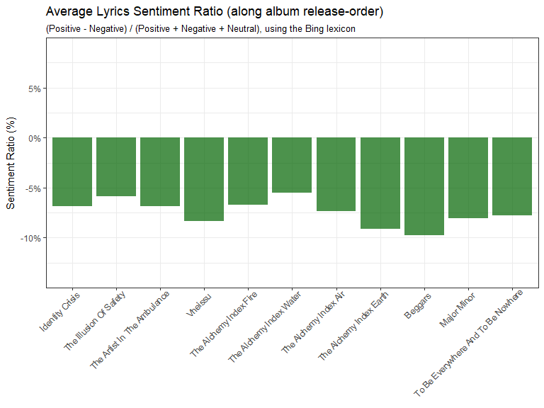
We’ve seen in previous plots that the sentiment of albums were more negative than positive and this plot confirms this as well. Why are Thrice’s lyrics categorized as negative as they are? From my experience a lot of Thrice’s songs are about acknowledging our struggles/sins/negatives and overcoming them, a more uplifting kind of vibe. Let’s look at how negative is defined by the three different lexicons.
Let’s compare the lexicons themselves on how many positive and negative words they each categorize.
get_sentiments("bing") %>%
  count(sentiment)
## # A tibble: 2 x 2
##   sentiment     n
##       <chr> <int>
## 1  negative  4782
## 2  positive  2006
get_sentiments("nrc") %>%
  count(sentiment)
## # A tibble: 10 x 2
##       sentiment     n
##           <chr> <int>
##  1        anger  1247
##  2 anticipation   839
##  3      disgust  1058
##  4         fear  1476
##  5          joy   689
##  6     negative  3324
##  7     positive  2312
##  8      sadness  1191
##  9     surprise   534
## 10        trust  1231
- In the Bing lexicon: there are 4782 words that can be categorized as negative along with 2006 positive words.
- In the NRC lexicon: there are 3324 words that can be categorized as negative along with 2312 positive words.
In the Bing lexicon, there are far more negative-categorized words than positive… more than twice as many in fact!
Now let’s count how many words in the lyrics were categorized for each sentiment:
emotions_lyrics_bing %>%
  group_by(sentiment) %>%
  summarize(sum = n())
## # A tibble: 3 x 2
##   sentiment   sum
##       <chr> <int>
## 1  negative   912
## 2   neutral  5095
## 3  positive   423
tidy_lyrics %>%
  left_join(get_sentiments("nrc"), by = "word") %>%
  group_by(sentiment) %>%
  summarize(sum = n())
## # A tibble: 11 x 2
##       sentiment   sum
##           <chr> <int>
##  1        anger   353
##  2 anticipation   425
##  3      disgust   244
##  4         fear   555
##  5          joy   455
##  6     negative   917
##  7     positive   846
##  8      sadness   570
##  9     surprise   235
## 10        trust   514
## 11         <NA>  4392
- In the lyrics (Bing): there are 912 negative words along with 423 positive words.
- In the lyrics (NRC): there are 917 negative words along with 846 positive words.
In summary, both the NRC and Bing lexicons didn’t have a category for most of the words in Thrice lyrics (neutral or NA) and there were more negative words than positive.
Let’s see if this holds true with the AFINN lexicon, the only lexicon we haven’t touched yet in the tidytext package! The AFINN lexicon gives a score from -5 (for negative sentiment) to +5 (positive sentiment).
emotions_lyrics_afinn <- tidy_lyrics %>%
  left_join(get_sentiments("afinn"), by = "word") %>%
  filter(!grepl('[0-9]', word))

emotions_lyrics_afinn %>%
  summarize(NAs= sum(is.na(score)))
##    NAs
## 1 5220
emotions_lyrics_afinn %>%
  select(score) %>%
  mutate(sentiment = if_else(score > 0, "positive", "negative", "NA")) %>%
  group_by(sentiment) %>%
  summarize(sum = n())
## # A tibble: 3 x 2
##   sentiment   sum
##       <chr> <int>
## 1        NA  5220
## 2  negative   696
## 3  positive   514
5220 of 6430 words in our lyrics data set don’t have AFINN score… With so many words in Thrice’s lyrics not categorized by any of these lexicons our results won’t be the most comprehensive, but these will have to do for now!
In line with the other lexicons, the majority of the words were categorized into NA (neutral)… then words were categorized as negative at a higher frequency compared to positive.
To create another visualization of lyrics sentiment, instead of taking the average for each album, we’ll just take the sentiment score for each album and plot it along each song. This way we’ll have more observations to compare the sentiment scoring ability of each lexicon.
afinn_scores <- emotions_lyrics_afinn %>%
  replace_na(replace = list(score = 0)) %>%
  group_by(index = title) %>%
  summarize(sentiment = sum(score)) %>%
  mutate(lexicon = "AFINN")

# combine the Bing and NRC lexicons into one data frame:

bing_nrc_scores <- bind_rows(
  tidy_lyrics %>%
    inner_join(get_sentiments("bing")) %>%
    mutate(lexicon = "Bing"),
  tidy_lyrics %>%
    inner_join(get_sentiments("nrc") %>%
                 filter(sentiment %in% c("positive", "negative"))) %>%
    mutate(lexicon = "NRC")) %>%
  # from here we count the sentiments, spread on positive/negative, then create the score:
  count(lexicon, index = title, sentiment) %>%
  spread(sentiment, n, fill = 0) %>%
  mutate(lexicon = as.factor(lexicon),
         sentiment = positive - negative)

all_lexicons <- bind_rows(afinn_scores, bing_nrc_scores)
lexicon_cols <- c("AFINN" = "#E41A1C", "NRC" = "#377EB8", "Bing" = "#4DAF4A")

all_lexicons %>%
  ggplot(aes(index, sentiment, fill = lexicon)) +
  geom_col(show.legend = FALSE) +
  facet_wrap(~lexicon, ncol = 1, scales = "free_y") +
  scale_fill_manual(values = lexicon_cols) +
  ggtitle("Comparison of Sentiments", subtitle = " Along Song-Order") +
  labs(x = "Index of All Thrice Songs", y = "Sentiment Score") +
  theme_bw() +
  theme(axis.text.x = element_blank())
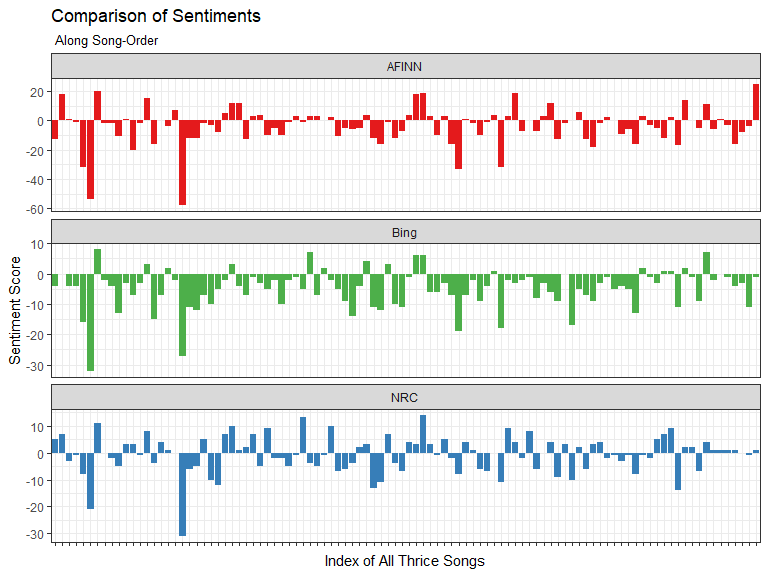
There are too many songs (103!) to show on the x-axis labels but I think you get the general idea!
The Bing lexicon sentiment along song order is generally negative, this lines up with what we saw in the average sentiment ratio plot where we had plotted along album order instead.
As we go through the songs from the first track on Identity Crisis, the eponymous “Identity Crisis”, all the way down to the last track on last year’s To Be Everywhere Is To Be Nowhere, “Salt And Shadow”, the AFINN, Bing, and NRC lexicons seem to agree on the sentiments but differ in the magnitude of the expressed sentiment for a each song.
The AFINN lexicon has the largest absolute magnitudes, however, remember that only 1210 out of 6430 total words in the lyrics were given a AFINN score. This means that the few words that do have scores exaggerate the magnitude of the sentiment scores relative to the other lexicons.
Keep in mind that the lexicons in the tidytext package are not the be all and end all for text/sentiment analysis. One can even create their own lexicons through crowd-sourcing (such as Amazon Mechanical-Turk, which is how some of the lexicons shown here were created), from utilizing word lists accrued by your own company throughout the years dealing with customer/employee feedback, etc. The sources are limitless!
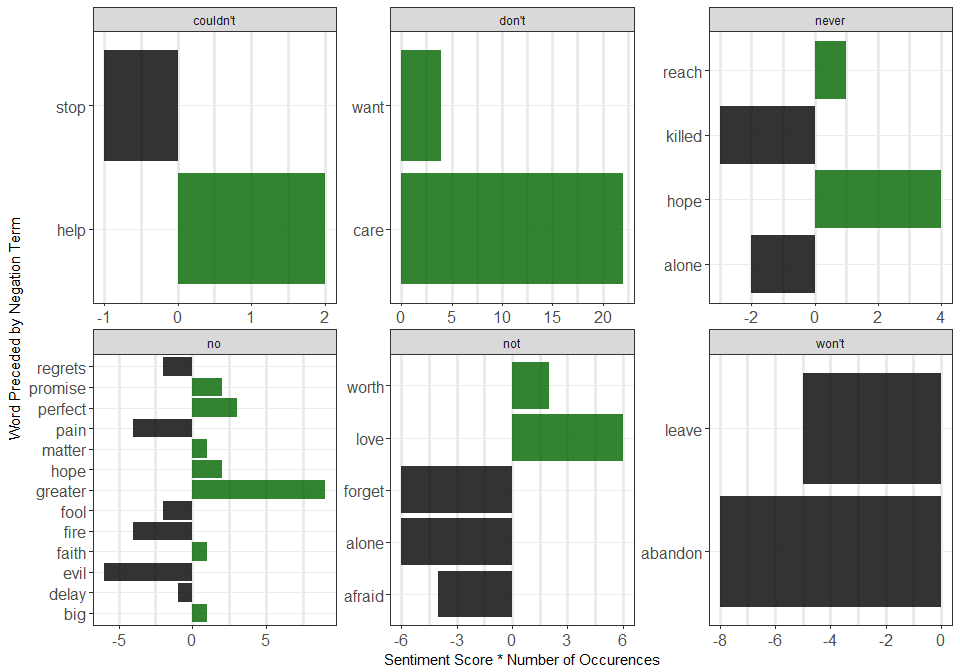
In the next article we’ll look at separating our lyrics into bi-grams (two words-per-row; which can then be split up into word1 and word2) and examining how the presence of negation words (“not”, “never”, “can’t”, “won’t”, etc.) is causing the lexicons to misclassify sentiments of the lyrics!
Preview for Part 4
Here’s a little preview of what examining negation words in bi-grams looks like. In the plot below we created a new variable called contribution where we multiplied the AFINN score of word2 (the word coming after a negation word word1) with their frequency to see the full effect of each negation bi-gram on the overall sentiment.