In Part 2 we will look at the lyrical content of the band, Thrice. By dividing the lyrics of each song into a single-word-per-row format, we can take a much closer look at the the lyrical content at various levels!
Let’s get started!
As always let’s load the various packages we are going to be using!
# Packages:
library(tidyverse)  # for dplyr, tidyr, ggplot2
library(tidytext)   # for separating text into words with unnest_tokens() function
library(stringr)    # for string detection, extraction, manipulation, etc.

library(gplots)     # for a certain type of plots not in ggplot2
library(ggrepel)    # for making sure labels don't overlap
library(scales)     # for fixing and tweaking the scales on graphs
library(gridExtra)  # for arranging multiple plots into a single page
First we have to load in the data set that we finished tidying up in Part 1 (not shown here).
Let’s finally take a look at the actual lyrics of Thrice.
df %>%
  select(lyrics) %>%
  substr(4, 116)
## [1] "Image marred by self-infliction <br> Private wars on my soul waged <br> Heart is scarred by dual volitions <br>"
Here we are looking at the first few lines of the first song in the first album (Identity Crisis (Live version)). We can see that the lyrics are separated into lines by the
tag. Note that this is how the lines were separated from the source, AZlyrics.com, and may not reflect how it is separated in the album booklets (as you can see, the first two lines shown above are actually one in the booklet).
For the purposes of this analysis and the slight discrepancy in the lines we will first break up the lyrics column into lines to get rid of the <br> tags and then split that line column so that the data is in the one-word-per-row format. This process is called tokenizing and we use the unnest_tokens() function in the tidytext package for restructuring text data sets!
Using unnest_tokens() we need to: - Enter in the output: the column to be created from tokenizing. - Enter in the input: the column that gets split or tokenized. - Enter in the token: the unit for tokenizing. Default is by “words”.
- Other inputs and options can be found by looking at the help page:
?unnest_tokens.
library(stringr)
# use the stringr for str_split() function to split "lyrics" on the <br> tags!

wordToken <-  df %>%
  unnest_tokens(output = line, input = lyrics, token = str_split, pattern = ' <br>') %>%
  unnest_tokens(output = word, input = line)

glimpse(wordToken)
## Observations: 18,757
## Variables: 9
## $ ID       <int> 1, 1, 1, 1, 1, 1, 1, 1, 1, 1, 1, 1, 1, 1, 1, 1, 1, 1,...
## $ album    <fctr> Identity Crisis, Identity Crisis, Identity Crisis, I...
## $ year     <int> 2000, 2000, 2000, 2000, 2000, 2000, 2000, 2000, 2000,...
## $ tracknum <int> 1, 1, 1, 1, 1, 1, 1, 1, 1, 1, 1, 1, 1, 1, 1, 1, 1, 1,...
## $ title    <chr> "Identity Crisis", "Identity Crisis", "Identity Crisi...
## $ writers  <chr> "Dustin Kensrue", "Dustin Kensrue", "Dustin Kensrue",...
## $ length   <S4: Period> 2M 58S, 2M 58S, 2M 58S, 2M 58S, 2M 58S, 2M 58S...
## $ lengthS  <S4: Period> 178S, 178S, 178S, 178S, 178S, 178S, 178S, 178S...
## $ word     <chr> "image", "marred", "by", "self", "infliction", "priva...
Now we have a data set with all words separated into individual rows.
Therefore, we can count how many times each word appears throughout the lyrics!
countWord <- wordToken %>% count(word, sort=TRUE)
countWord  %>% head(10)
## # A tibble: 10 x 2
##     word     n
##    <chr> <int>
##  1   the   864
##  2   and   609
##  3     i   582
##  4    to   400
##  5   you   373
##  6    we   335
##  7     a   333
##  8    of   296
##  9    in   273
## 10    my   251
Just from looking at this it is clear that this isn’t very informative about the content of lyrics. Words such as “I”, “you”, “we”, “very”, “the” aren’t very useful for analyzing the meaningfulness of our data set. These very common set of words are called “stop words”. For example:
data("stop_words")

set.seed(1)
sample_stop <- stop_words %>% sample_n(10)

sample_stop
## # A tibble: 10 x 2
##       word  lexicon
##      <chr>    <chr>
##  1   noone    SMART
##  2   thank    SMART
##  3  hadn't snowball
##  4 several     onix
##  5    into    SMART
##  6    said     onix
##  7   think     onix
##  8   alone     onix
##  9    then snowball
## 10    best    SMART
Using the built-in lexicons (“onix”, “SMART”, and “snowball”) in the tidytext package we can create a new data set where we filter out these “stop words” from our word column in wordToken.
This can be done by using anti_join() function which returns all rows from x (our original wordtoken data set) where there are no matching values in y (stop_words data set) on a variable with a common name across both data sets (word).
wordToken2 <- wordToken %>%
  anti_join(stop_words) %>% # Take out rows of `word` in wordToken that appear in stop_words
  arrange(ID)               # Can also arrange by track_num, basically the same thing

countWord2 <- wordToken2 %>% count(word, sort = TRUE)

countWord2 %>% head(10)
## # A tibble: 10 x 2
##     word     n
##    <chr> <int>
##  1  eyes    73
##  2  love    64
##  3 light    53
##  4 blood    43
##  5  life    43
##  6  fall    37
##  7 world    35
##  8  time    32
##  9 heart    31
## 10  hold    30
With “stop words” being filtered out of our data set, “eyes”, “love”, “light”, “blood”, and “life” are the most common! We can make much more inferences about the lyrics from those compared to “I”, “the”, “and”, and “to”!
Now that we have one data set with “stop words” and one without, we can compare them to really emphasize the importance of filtering out “stop words” from any text data:
# graph of most common words (including stop words)
one <- countWord %>% head(10) %>%
  ggplot(aes(reorder(word, n), n)) +
  geom_bar(stat = "identity", fill = "darkgreen", alpha = 0.75) +
  ggtitle("Comparison of 'Most Common Words'") +
  labs(x = "With 'stop words'", y = "Frequency") +
  scale_y_continuous(breaks = pretty_breaks(5)) +
  coord_flip() +
  theme_bw() +
  theme(panel.grid.major.x = element_line(size = 1.25),
        axis.text.x = element_text(size = 12, face = "bold"),
        plot.title = element_text(hjust = 0.5))

# graph of most common words (no stop words)
two <- countWord2 %>% head(10) %>%
  ggplot(aes(reorder(word, n), n)) +
  geom_bar(stat = "identity", fill = "darkgreen", alpha = 0.75) +
  labs(x = "No 'stop words'", y = "Frequency") +
  scale_y_continuous(breaks = pretty_breaks()) +
  coord_flip() +
  theme_bw() +
  theme(panel.grid.major.x = element_line(size = 1.25),
        axis.text.x = element_text(size = 12, face = "bold"))

grid.arrange(one, two)

You can clearly see the difference between the data sets!
The fact that the scales for frequency are very different between the plots shows how individually meaningless “stop words” such as “the”, “and”, “to”, and “a” can really disrupt our analysis. The plot without “stop words” gives us a much clearer idea of the most common and meaningful words in Thrice’s lyrics!
Another way to see this effect is by visualizing our data in a different way, using word clouds!
library(wordcloud)
layout(matrix(c(1,2),1,2, byrow = TRUE))

wordcloud(words = countWord$word, freq = countWord$n, random.order = FALSE, max.words = 300,
          colors = brewer.pal(8, "Dark2"), use.r.layout = TRUE)

wordcloud(countWord2$word, countWord2$n, random.order = FALSE, max.words = 300,
          colors = brewer.pal(8, "Dark2"), use.r.layout = TRUE)

With the word cloud visualization, we can really tell how the “stop words” in the left cloud obscures or “crowds out” all of the other more meaningful words due to the sheer amount of “the”s, “you”s, and “to”s that appear in the lyrics text.
Data exploration
Now that we’ve spread out each word into it’s own row, let’s take a closer look at our new data sets!
wordToken %>% select(title) %>% n_distinct()
## [1] 100
wordToken2 %>% select(title) %>% n_distinct()
## [1] 100
Both wordToken and wordToken2 give the number of songs at 100… but wait! In Part 1 we checked that there were a total of 103 songs, in these “tokenized” data sets the instrumental songs were not included simply because as they do not have any words, so there is no row for those instrumentals to exist in these data sets!
df %>% summarise(num_songs = n()) # 103 songs in total, as each row = 1 song in original data set
##   num_songs
## 1       103
Let’s look at the exact number of unique words in Thrice’s lyrics. As almost 100% of Thrice’s songs are written by Dustin Kensrue, we’ll be able to see just how extensive his vocabulary is!
wordToken %>% select(word) %>% n_distinct()
## [1] 2480
2480! Not bad, let’s take out all the “stop words” though…
wordToken2 %>% select(word) %>% n_distinct()
## [1] 2095
2095 unique and non-“stop word” words in Thrice’s lyrics! Which also means in wordToken2 we took out around 400 distinct “stop words” out from wordToken.
Lyrics exploration
Now let’s create a new data set called WordsPerSong to create a histogram of the distribution of songs by the number of words (including “stop words”).
# WordsPerSong
WordsPerSong <- wordToken %>%
  group_by(title) %>%
  summarize(wordcounts = n()) %>%    # each row = 1 word
  arrange(desc(wordcounts))

WordsPerSong %>%
  ggplot(aes(x = wordcounts)) +
  geom_histogram(bins = 50, color = "white", fill = "darkgreen") +
  geom_vline(xintercept = median(WordsPerSong$wordcounts),
             color = "red", linetype = "dashed", size = 1.25) +
  scale_y_continuous(breaks = pretty_breaks(), expand = c(0, 0), limits = c(0, 12)) +
  scale_x_continuous(breaks = pretty_breaks(10), expand = c(0, 0), limits = c(0, 410)) +
  xlab('Total # of Words') +
  ylab('# of Songs') +
  labs(title = 'Distribution of Songs by Number of Words \n (Dashed red line: median)') +
  theme_bw() +
  theme(panel.grid.minor = element_blank(),
        plot.title = element_text(hjust = 0.5))
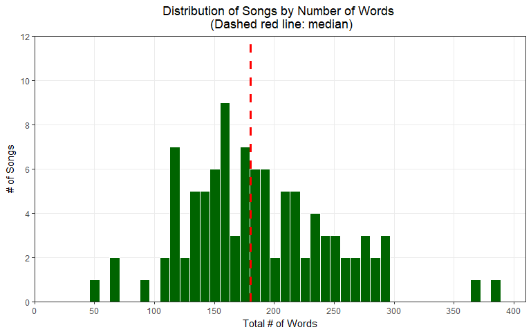
The wordToken and wordToken2 data sets unfortunately filters out the instrumentals all together, as the rows for the instrumentals are not created by the unnest_tokens() function. Therefore, the median and mean values for word count will be slightly off in both the wordToken and wordToken2 data sets.
Count the number of songs for each album, we did this in Part 1 with df, this time let’s use the wordToken2 data set that we just created:
wordToken2 %>%
  group_by(album) %>%
  summarize(num_songs = n_distinct(title)) %>%
  arrange(desc(num_songs))
## # A tibble: 11 x 2
##                                 album num_songs
##                                <fctr>     <int>
##  1             The Illusion Of Safety        13
##  2        The Artist In The Ambulance        12
##  3                            Vheissu        11
##  4                        Major Minor        11
##  5                    Identity Crisis        10
##  6                            Beggars        10
##  7 To Be Everywhere And To Be Nowhere        10
##  8             The Alchemy Index Fire         6
##  9              The Alchemy Index Air         6
## 10            The Alchemy Index Earth         6
## 11            The Alchemy Index Water         5
Let’s dig deeper, what about the number of words per song? We need to use wordToken instead of df or wordToken2 as “stop_words” should be included for the total word sum.
wordToken %>%
  select(title, album, word) %>%
  group_by(title, album) %>%
  summarize(num_word = n()) %>%
  arrange(desc(num_word)) %>%
  head(10)
## # A tibble: 10 x 3
## # Groups:   title [10]
##                          title                              album num_word
##                          <chr>                             <fctr>    <int>
##  1                  The Weight                            Beggars      383
##  2                 Black Honey To Be Everywhere And To Be Nowhere      365
##  3                     Wake Up To Be Everywhere And To Be Nowhere      297
##  4                   Under Par                    Identity Crisis      293
##  5                Stay With Me To Be Everywhere And To Be Nowhere      292
##  6                The Arsonist             The Alchemy Index Fire      284
##  7          The Sky Is Falling              The Alchemy Index Air      281
##  8           Blood On The Sand To Be Everywhere And To Be Nowhere      280
##  9 The Artist In The Ambulance        The Artist In The Ambulance      279
## 10                    Daedalus              The Alchemy Index Air      273
How about words per album? Let’s also turn this info into a bar graph!
wordToken %>%
  select(album, word) %>%
  group_by(album) %>%
  summarize(num_word = n()) %>%
  arrange(desc(num_word)) %>%
  ggplot(aes(reorder(album, num_word), num_word, fill = num_word)) +
  geom_bar(stat = "identity") +
  scale_y_continuous(expand = c(0.01, 0)) +
  scale_fill_gradient(low = "#a1d99b", high = "#006d2c", guide = FALSE) +
  coord_flip() +
  theme_bw() +
  theme(axis.text.y = element_text(size = 8), axis.title.y = element_blank()) +
  ylab("Number of Words")
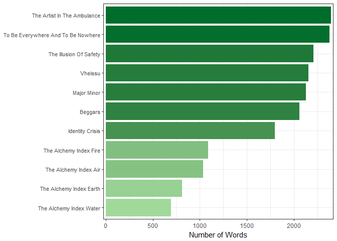
Individually, the Alchemy Index albums are the lowest as they each have only six songs each, if they were combined into their actual album sets (Volume 1: Fire & Water, Volume 2: Earth & Air), they would probably have more words than Identity Crisis.
Some more exploration with dplyr verbs!
Let’s use filter() to look at a specific album or specific song.
wordToken %>%
  filter(album == "Vheissu") %>%
  summarize(num_word = n())
##   num_word
## 1     2155
wordToken %>%
  filter(title == "The Weight") %>%
  summarize(num_word = n())
##   num_word
## 1      383
The Weight was the first Thrice song I listened to in my friend’s dorm room back in college, so it has quite a sentimental value to me! So let’s look at the most common words in the lyrics for The Weight!
wordToken2 %>%
  filter(title == "The Weight") %>%
  group_by(title) %>%
  count(word) %>%
  arrange(desc(n)) %>%
  head(5)
## # A tibble: 5 x 3
## # Groups: title [1]
## title word n
## <chr> <chr> <int>
## 1 The Weight wont 15
## 2 The Weight leave 9
## 3 The Weight love 6
## 4 The Weight abandon 4
## 5 The Weight burning 4
From the Top 5 most common words, “won’t”, “leave”, “love”, “abandon”, “burning”, it is clear that this song is about love and commitment. Indeed, the “won’t” in this song is only used in a positive sense, such as “I won’t abandon you” and “I won’t leave you high and dry” reinforcing Dustin’s message that love is a huge commitment; the title of the song, The Weight, actually refers to the gravity and seriousness of that commitment.
We can also combine dplyr with other functions, such as various stringr functions to find specific words! Let’s take a closer look at one of the most common words that we found, “light”, and check the total number of times “light” appears in lyrics of song.
wordToken2 %>%
  str_count("light") %>%
  sum()
## [1] 87
We can see that across all the songs in Thrice’s discography, the word “light” shows up 87 times!
Now we use mutate() to create a new column that gives us the number of times the word “light” appears for each song.
wordToken2 %>%
  select(title, album, word) %>%
  mutate(light = str_count(word, "light")) %>%
  group_by(title, album) %>%
  summarize(total_light = sum(light)) %>%
  arrange(desc(total_light)) %>%
  head(5)
## # A tibble: 5 x 3
## # Groups:   title [5]
##                              title                              album
##                              <chr>                             <fctr>
## 1 Between The End And Where We Lie                            Vheissu
## 2                        Music Box                            Vheissu
## 3      The Artist In The Ambulance        The Artist In The Ambulance
## 4                       The Window To Be Everywhere And To Be Nowhere
## 5      A Song For Milly Michaelson              The Alchemy Index Air
## # ... with 1 more variables: total_light <int>
Let’s look at the proportion of “light” out of all the words in Thrice’s lyrics!
wordToken %>%
  select(title, album, word) %>%
  summarize(light = str_count(word, "light") %>% sum(),
            num_word = n(),
            prop_light = (light / num_word))
##   light num_word  prop_light
## 1    87    18757 0.004638268
Even one of the most common words, “light”, accounts for only 0.46% of all the words in the lyrics of Thrice’s songs!
What about the most frequent word in a specific song (with and without “stop words”)?
wordToken %>%
  group_by(title) %>%
  count(word) %>%
  arrange(desc(n)) %>%
  head(10)
## # A tibble: 10 x 3
## # Groups:   title [9]
##                     title  word     n
##                     <chr> <chr> <int>
##  1            Black Honey     i    48
##  2 Image Of The Invisible   the    36
##  3        All That's Left    we    35
##  4 Image Of The Invisible    we    27
##  5           Yellow Belly   you    25
##  6                Wake Up    we    24
##  7               Promises    we    23
##  8             The Weight     i    22
##  9                Blinded     i    21
## 10          In Your Hands     i    21
The most common words seem to mainly be personal nouns along with “the”.
wordToken2 %>%
  group_by(title) %>%
  count(word, sort = TRUE) %>%
  head(10)
## # A tibble: 10 x 3
## # Groups: title [8]
## title word n
## <chr> <chr> <int>
## 1 Black Honey ill 20
## 2 Wake Up gotta 17
## 3 Wake Up wake 17
## 4 Yellow Belly dont 16
## 5 The Weight wont 15
## 6 Image Of The Invisible image 13
## 7 Image Of The Invisible invisible 13
## 8 The Earth Isn't Humming fall 13
## 9 Blood On The Sand sick 12
## 10 Between The End And Where We Lie daylight 11
“I’ll” and “I” appears the most in both lists from the song, Black Honey, a very political song that is an allegory for the meddling foreign policy of the United States. The constant appearance of “I”, “I’ll”, “I’ve” throughout the song highlights the very selfish, arrogant, and oblivious nature of the protagonist, who is aggressively seeking to obtain the “black honey”, referring to the petroleum of Middle Eastern countries.
wordToken2 %>%
  filter(title == "Black Honey") %>%
  count(word, sort = TRUE) %>%
  head(10)
## # A tibble: 10 x 2
## word n
## <chr> <int>
## 1 ill 20
## 2 bees 5
## 3 hand 5
## 4 swarm 5
## 5 swinging 5
## 6 till 5
## 7 theyre 4
## 8 time 4
## 9 understand 4
## 10 dont 3
In second place for this song is “bees”. In this song the the “bees” and “hornets”, symbolize the inhabitants of the Middle East countries that are trampled in the protagonist’s pursuit for the “black honey”. It’s a really great song (have a listen here), my second favorite off the album after Hurricane.
Back to the overall word count, the appearance of “image” and “invisible” from the song Image of the Invisible is more straightforward as it is shouted out during the chorus repeatedly. Most of that song is Thrice screaming that title phrase out actually!
From looking at this data, a thing to consider is that the data can be skewed toward repeated phrases in a song, like the chorus! From other lyrics analysis I’ve seen, people have tried to find lyrics that don’t have repeated choruses, however, most lyrics websites aren’t well moderated or have a ton of different people with different input styles posting lyrics of different songs for a single artist so it can be a bit tricky in this regard.
Creating nested data frames for storing plots for each album.
Now let’s try to create plots for the most frequent words for each album. To do this we need to create a “nested” data set. Basically, the “data” column will contain the specific list of the most common words for each individual album (row).
# most frequent unigrams per album: ####

word_count_nested <- wordToken2 %>%
  group_by(album, word) %>%
  summarize(count = n(), sort = TRUE) %>%
  top_n(5, wt = count) %>%
  arrange(album, desc(count)) %>%
  nest()
Let’s take a look at the individual elements of our new “data” column!
word_count_nested$data[[1]]
## # A tibble: 8 x 3
##    word count  sort
##   <chr> <int> <lgl>
## 1 heart    12  TRUE
## 2  eyes     8  TRUE
## 3  life     6  TRUE
## 4 light     6  TRUE
## 5   cry     5  TRUE
## 6 faith     5  TRUE
## 7  soul     5  TRUE
## 8  true     5  TRUE
word_count_nested$data[[5]]
## # A tibble: 5 x 3
##    word count  sort
##   <chr> <int> <lgl>
## 1  free    15  TRUE
## 2  burn    13  TRUE
## 3  send    11  TRUE
## 4  fire    10  TRUE
## 5 flame     9  TRUE
The most common word for the first list (Album = Identity Crisis) is “heart” and the fifth list (Album = AI: Fire) is “free”. The only problem with the top_n() function is that if there are ties than the total number will be bigger than the specified n such as in Identity Crisis above.
Now we use the data to create a plot for each album using the map2() function which allows us to iteratively create a plot from each specific data column from each album row and stores the plot information in its own column plot, just like we did in data.
word_count_nested <- word_count_nested %>%
  mutate(plot = map2(data, album,
                     ~ggplot(data = .x, aes(fill = count)) +
           geom_bar(aes(reorder(word, count), count),
                    stat = "identity", width = 0.65) +
           scale_y_continuous(breaks = pretty_breaks(10), limits = c(0, 22), expand = c(0, 0)) +
           scale_fill_gradient(low = "#a1d99b", high = "#006d2c", guide = FALSE) +
           ggtitle(.y) +
           labs(x = NULL, y = NULL) +
           coord_flip() +
           theme_bw() +
           theme(axis.text.y = element_text(size = 7),
                 title = element_text(size = 10))
           ))

str(word_count_nested, list.len = 3, max.level = 2)
## Classes 'tbl_df', 'tbl' and 'data.frame':    11 obs. of  3 variables:
##  $ album: Factor w/ 11 levels "Identity Crisis",..: 1 2 3 4 5 6 7 8 9 10 ...
##  $ data :List of 11
##   ..$ :Classes 'tbl_df', 'tbl' and 'data.frame': 8 obs. of  3 variables:
##   ..$ :Classes 'tbl_df', 'tbl' and 'data.frame': 7 obs. of  3 variables:
##   ..$ :Classes 'tbl_df', 'tbl' and 'data.frame': 6 obs. of  3 variables:
##   .. [list output truncated]
##  $ plot :List of 11
##   ..$ :List of 9
##   .. ..- attr(*, "class")= chr  "gg" "ggplot"
##   ..$ :List of 9
##   .. ..- attr(*, "class")= chr  "gg" "ggplot"
##   ..$ :List of 9
##   .. ..- attr(*, "class")= chr  "gg" "ggplot"
##   .. [list output truncated]
On inspection, the word_count_nested data frame consists of three columns of album, data, and plot by 11 rows, one row for each album. The column data is a series of lists that holds the Top 10 or so words for each album (row). For example, the first element of data is a data frame of eight observations of two variables, specifically the eight most common words in the first album as rows with word and count as the two column variables. The next column, plot, is a series of lists that holds the plot information (the ggplot2 code we added into the data frame with mutate()) for each album (row).
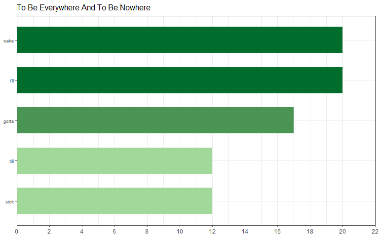
By selecting the specific element within the list, we can extract the plot for a certain album
word_count_nested$plot[[2]]
word_count_nested$plot[[11]]
With everything organized in a “tidy” way, let’s try to plot for all of the albums!
First let’s try with something we used in Part 1, facetting!
Before we start plotting we need to “unnest” the information inside the data column to create our facetted plot. Then we can use our regular ggplot commands to create our facetted plot along with facet_grid().
word_count_nested %>%
  unnest(data) %>%                   # take data out from list
  ggplot(aes(x = word, y = count)) +
  geom_bar(stat = "identity") +
  facet_grid(.~album)
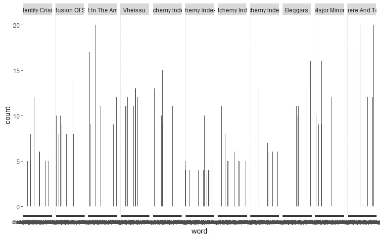
Regardless of the fact that we don’t have enough screen space, facetting is clearly not the way to do this. One way to solve our problem is to code in a way that each plot for each album is printed out individually and then to arrange all those individual plots onto one page. This way the group of plots won’t be forcibly squished together into one gigantic plot.
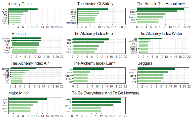
One way is to use a base R method with the do.call() function. This will iterate the grid.arrange() function for the ggplot data stored in plot in every row/album.
do.call(grid.arrange, c(word_count_nested$plot, ncol = 3))
Another way is to save all the plotting data in the plot column into a single list… To get an output slightly different from the above, for this list of plots let’s make a subset of the 1st to 4th plots (Albums: Identity Crisis to The Artist In The Ambulance) instead.
nested_plots <- word_count_nested$plot[1:4]
str(nested_plots, list.len = 2, max.level = 2)
## List of 4
##  $ :List of 9
##   ..$ data       :Classes 'tbl_df', 'tbl' and 'data.frame':  8 obs. of  3 variables:
##   ..$ layers     :List of 1
##   .. [list output truncated]
##   ..- attr(*, "class")= chr [1:2] "gg" "ggplot"
##  $ :List of 9
##   ..$ data       :Classes 'tbl_df', 'tbl' and 'data.frame':  7 obs. of  3 variables:
##   ..$ layers     :List of 1
##   .. [list output truncated]
##   ..- attr(*, "class")= chr [1:2] "gg" "ggplot"
##   [list output truncated]
From inspecting the list with str(), we can see that this is a list with a length of four, basically one list for each of the four albums that we subsetted. Within each album’s list we have another set of lists for the respective data and plot elements! Using this list of lists we can pass it through the plot_grid() function from the cowplot package to arrange multiple plots on a single page. In this function we basically call our list of plots with the plotlist = argument and then we can also specify the number of columns, rows, label size, etc.
library(cowplot)

plot_grid(plotlist = nested_plots, ncol = 2)
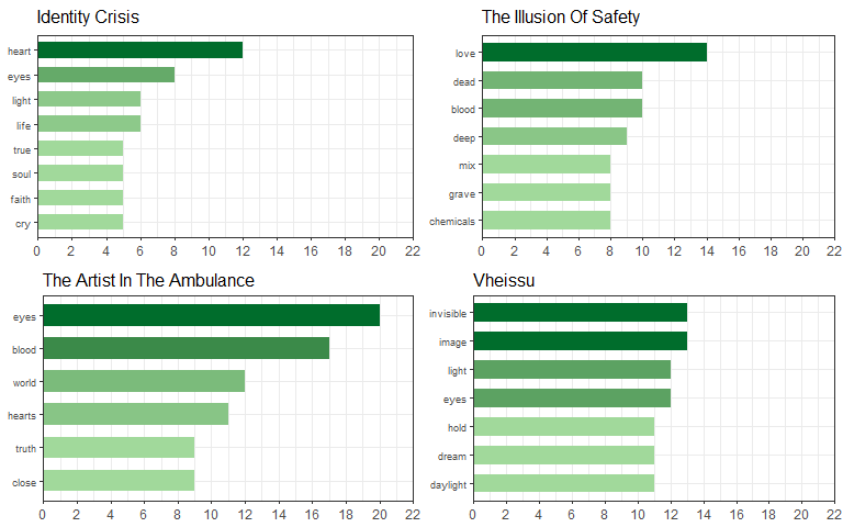
We can now view all the plots (or a subset of them) on a single page!
By using the map2() function from purrr package, this time we apply the function ggsave() so that it iteratively saves the plot for each album!
map2(paste0(word_count_nested$album, ".pdf"), word_count_nested$plot, ggsave)
We can check that the code ran properly (without having to manually look into your working directory) with the file.exists() function.
file.exists(paste0(word_count_nested$album, ".pdf"))
## [1] TRUE TRUE TRUE TRUE TRUE TRUE TRUE TRUE TRUE TRUE TRUE
With all those plots properly saved into separate files we can now share and send them to other people!
Today we did divided up the lyrics into singular words and analyzed it at various levels and through various filters. In Part 3 we will look more closely at the different sentiments/emotions that are expressed in Thrice’s lyrics!
(Link: Part 3)
(10/30/2017 EDIT: forgot the wt = argument in top_n() when nesting the dataframe, each nested data column should have the proper number of rows now!)