I recently came across a cool waffle viz for the top 20 shot-creating action players in the big 5 European soccer leagues done by Harsh Krishna on Twitter, see original Tweet here. He also posted the code in this Github gist with a call for help in solving an issue he was having with the preserving the sum of a group of metrics after rounding the individual metrics to integers. Below is the code he posted in full. The problem in particular is after the second for loop where he rounds the metrics, he finds that the sum of the metrics don’t add up to 100(%). His way of resolving this was choosing the Sh_SCA variable and trying to manipulate the values in that metric until the total summed back up to 100.

# Harsh Krishna `@placeholder2004`
# https://github.com/harshkrishna17/R-Code/blob/main/Waffle.R
# Libraries

library(tidyverse)
library(worldfootballR)
library(ggtext)
library(extrafont)
library(waffle)
library(MetBrewer)

# Scraping

data <- fb_big5_advanced_season_stats(season_end_year = 2022, stat_type = "gca", team_or_player = "player")

# Data Wrangling 

data1 <- data %>%
  filter(Mins_Per_90 >= 9) %>%
  select(Player, Mins_Per_90, SCA90_SCA, SCA_SCA, PassLive_SCA, PassDead_SCA, Drib_SCA, Sh_SCA, Fld_SCA, Def_SCA)

data1 <- data1[order(as.numeric(data1$SCA90_SCA),decreasing = TRUE),]
data1 <- data1[c(1:20),]

df <- data1[order(as.numeric(data1$SCA90_SCA),decreasing = TRUE),]
df <- df[c(1:20),]

Player <- data1$Player
Mins <- data1$Mins_Per_90
data1 <- subset(data1, select = -c(Player, Mins_Per_90, SCA90_SCA))

for(i in 1:ncol(data1)) {
  data1[, i] <- data1[, i] / Mins
}

SCA <- data1$SCA_SCA 

for(i in 1:ncol(data1)) {
  data1[, i] <- round((data1[, i] / SCA) * 100, 0)
}

data1 <- data1 %>%
  mutate(Total = PassLive_SCA + PassDead_SCA + Drib_SCA + Sh_SCA + Fld_SCA + Def_SCA)

## run this ifelse statement as many times as necessary until the Total comes out to be a 100 for all rows.
data1 <- data1 %>% mutate(Sh_SCA = ifelse(Total == 100, Sh_SCA,
                                          ifelse(Total < 100, Sh_SCA + 1,
                                                 ifelse(Total > 100, Sh_SCA - 1, NA)))) %>% 
  mutate(Total = PassLive_SCA + PassDead_SCA + Drib_SCA + Sh_SCA + Fld_SCA + Def_SCA)

data1$Player <- Player 

data1 <- data1 %>%
  pivot_longer(!Player, values_to = "SCAp90", names_to = "SCATypes") %>%
  filter(!SCATypes == "SCA_SCA") %>%
  filter(!SCATypes == "Total") %>%
  count(Player, SCATypes, wt = SCAp90)

data1$Player <- factor(data1$Player, levels = print(df$Player))

# Custom theme function

theme_athletic <- function() {
  theme_minimal() +
    theme(plot.background = element_rect(colour = "#151515", fill = "#151515"),
          panel.background = element_rect(colour = "#151515", fill = "#151515")) +
    theme(plot.title = element_text(colour = "white", size = 24, family = "Fried Chicken Bold", hjust = 0.5),
          plot.subtitle = element_markdown(colour = "#525252", size = 18, hjust = 0.5),
          plot.caption = element_text(colour = "white", size = 15, hjust = 1),
          axis.title.x = element_text(colour = "white", face = "bold", size = 14),
          axis.title.y = element_text(colour = "white", face = "bold", size = 14),
          axis.text.x = element_blank(),
          axis.text.y = element_blank()) +
    theme(panel.grid.major = element_blank(),
          panel.grid.minor = element_blank(),
          panel.background = element_blank()) +
    theme(legend.title = element_text(colour = "white"),
          legend.text = element_text(colour = "white"))
}

# Plotting

data1 %>%
  ggplot(aes(fill = SCATypes, values = n)) +
  geom_waffle(nrows = 10, size = 1.5, colour = "#151515", flip = TRUE) +
  scale_fill_manual(values = met.brewer(name = "Gauguin", n = 6, type = "discrete")) +
  facet_wrap(~Player) +
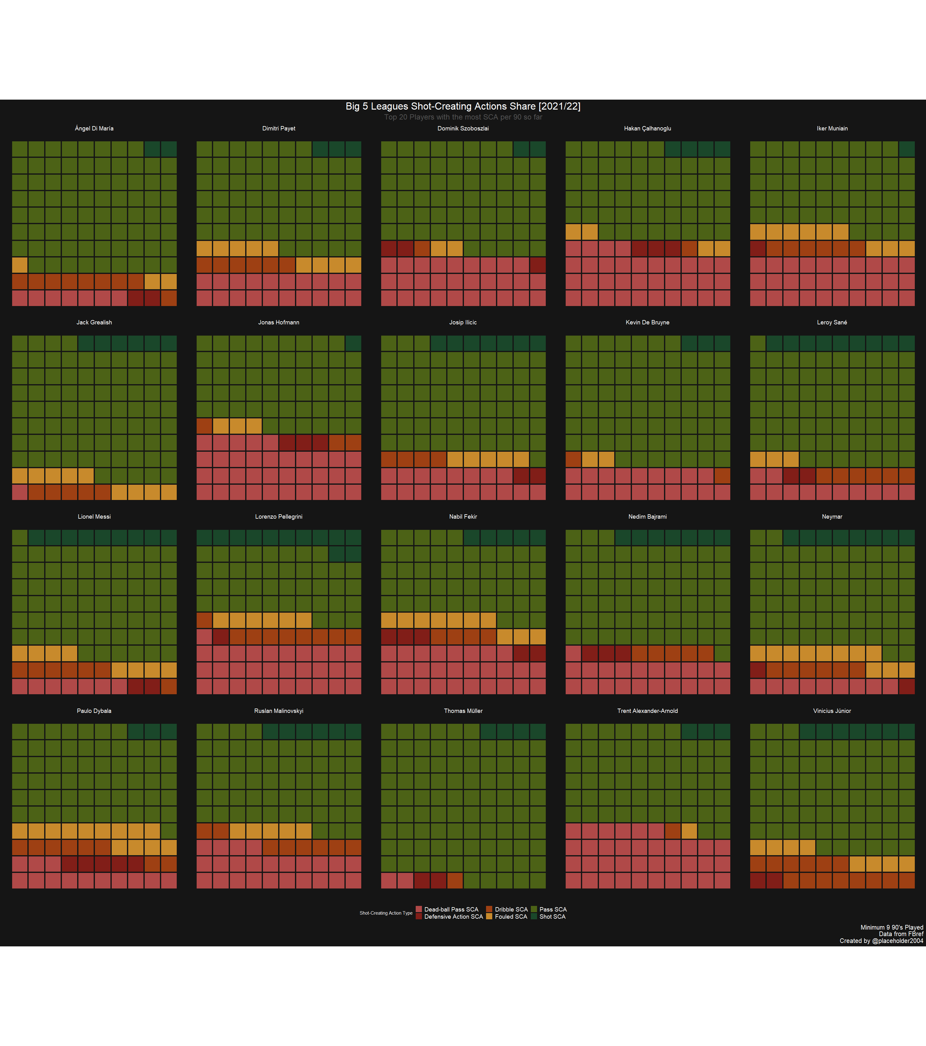
  labs(title = "Big 5 Leagues Shot-Creating Actions Share [2021/22]",
       subtitle = "Top 20 Players with the most SCA per 90 so far",
       caption = "Minimum 9 90's Played\nData from FBref\nCreated by @placeholder2004") +
  theme_athletic() +
  theme(aspect.ratio = 1,
        strip.background = element_blank(),
        strip.text = element_text(colour = "white", size = 14),
        legend.position = "bottom",
        legend.text = element_text(size = 14))

# Save

setwd("C:/Users/harsh_1mwi2o4/Downloads")
ggsave("wafflebig5.png", width = 3100, height = 3500, units = "px")

This is a problem I’ve faced in the past and I’m sure many others have too, whether in the context of soccer analysis or otherwise. So I decided to tackle this problem as a fun coding challenge using the tidyverse!

Let’s get started!

Packages

I prefer typing out the specific tidyverse packages rather than loading everything in at once.

library(dplyr)
library(tidyr)
library(worldfootballR)
library(ggtext)
library(extrafont)
library(waffle)
library(MetBrewer)

Scrape data

Get data from FBref/StatsBomb with the {worldfootballR} package.

# Scraping
data_raw <- fb_big5_advanced_season_stats(season_end_year = 2022, stat_type = "gca", team_or_player = "player")

glimpse(data_raw)

## Rows: 2,540
## Columns: 27
## $ X               <int> 1, 2, 3, 4, 5, 6, 7, 8, 9, 10, 11, 12, 13, 14, 15, 16,~
## $ Season_End_Year <int> 2022, 2022, 2022, 2022, 2022, 2022, 2022, 2022, 2022, ~
## $ Squad           <chr> "Alavés", "Alavés", "Alavés", "Alavés", "Alavés", "Ala~
## $ Comp            <chr> "La Liga", "La Liga", "La Liga", "La Liga", "La Liga",~
## $ Player          <chr> "Martin Agirregabiria", "Mircea Alexandru Tirlea", "Ru~
## $ Nation          <chr> "ESP", "ROU", "ESP", "ARG", "ESP", "ESP", "SWE", "ESP"~
## $ Pos             <chr> "DF", "DF", "DF", "MF", "MF", "FW", "FW,MF", "MF", "FW~
## $ Age             <chr> "25-249", "21-292", "26-088", "28-293", "24-012", "27-~
## $ Born            <int> 1996, 2000, 1995, 1993, 1998, 1994, 1992, 1994, 1990, ~
## $ Mins_Per_90     <dbl> 13.6, 0.2, 16.4, 0.6, 7.6, 0.0, 3.0, 0.4, 18.5, 17.9, ~
## $ SCA_SCA         <int> 22, 0, 23, 0, 23, 0, 10, 1, 40, 3, 4, 5, 2, 12, 3, 11,~
## $ SCA90_SCA       <dbl> 1.62, 0.00, 1.40, 0.00, 3.02, 0.00, 3.28, 2.25, 2.16, ~
## $ PassLive_SCA    <int> 16, 0, 11, 0, 12, 0, 5, 1, 24, 0, 4, 3, 2, 10, 1, 6, 4~
## $ PassDead_SCA    <int> 2, 0, 9, 0, 8, 0, 0, 0, 1, 2, 0, 1, 0, 0, 0, 0, 18, 0,~
## $ Drib_SCA        <int> 1, 0, 0, 0, 1, 0, 1, 0, 1, 0, 0, 1, 0, 2, 0, 1, 1, 0, ~
## $ Sh_SCA          <int> 0, 0, 0, 0, 1, 0, 0, 0, 6, 1, 0, 0, 0, 0, 2, 0, 1, 2, ~
## $ Fld_SCA         <int> 3, 0, 2, 0, 1, 0, 2, 0, 6, 0, 0, 0, 0, 0, 0, 3, 0, 1, ~
## $ Def_SCA         <int> 0, 0, 1, 0, 0, 0, 2, 0, 2, 0, 0, 0, 0, 0, 0, 1, 1, 0, ~
## $ GCA_GCA         <int> 2, 0, 3, 0, 0, 0, 3, 0, 5, 1, 0, 1, 0, 0, 0, 3, 3, 0, ~
## $ GCA90_GCA       <dbl> 0.15, 0.00, 0.18, 0.00, 0.00, 0.00, 0.99, 0.00, 0.27, ~
## $ PassLive_GCA    <int> 1, 0, 0, 0, 0, 0, 1, 0, 2, 0, 0, 1, 0, 0, 0, 1, 1, 0, ~
## $ PassDead_GCA    <int> 0, 0, 2, 0, 0, 0, 0, 0, 0, 0, 0, 0, 0, 0, 0, 0, 1, 0, ~
## $ Drib_GCA        <int> 1, 0, 0, 0, 0, 0, 0, 0, 0, 0, 0, 0, 0, 0, 0, 0, 0, 0, ~
## $ Sh_GCA          <int> 0, 0, 0, 0, 0, 0, 0, 0, 1, 1, 0, 0, 0, 0, 0, 0, 1, 0, ~
## $ Fld_GCA         <int> 0, 0, 1, 0, 0, 0, 1, 0, 1, 0, 0, 0, 0, 0, 0, 1, 0, 0, ~
## $ Def_GCA         <int> 0, 0, 0, 0, 0, 0, 1, 0, 1, 0, 0, 0, 0, 0, 0, 1, 0, 0, ~
## $ Url             <chr> "https://fbref.com/en/players/355c883a/Martin-Agirrega~

Instead of ordering and subsetting with base functions in the original, I used arrange() and slice() to grab the top 20 players by SCA per 90.

# Data Wrangling 
df1 <- data_raw %>%
  filter(Mins_Per_90 >= 9) %>%
  ## use contains() so I don't have to type out every `SCA` variable out
  select(Player, Mins_Per_90, contains("SCA")) %>% 
  ## arrange by SCA per 90 (descending) then take top 20 rows
  arrange(desc(SCA90_SCA)) %>%
  slice(1:20)

glimpse(df1)

## Rows: 20
## Columns: 10
## $ Player       <chr> "Dimitri Payet", "Lorenzo Pellegrini", "Hakan Çalhanoglu"~
## $ Mins_Per_90  <dbl> 15.4, 13.8, 12.7, 9.2, 12.2, 9.2, 10.3, 9.6, 11.8, 17.3, ~
## $ SCA_SCA      <int> 115, 83, 76, 55, 72, 53, 59, 55, 66, 94, 66, 89, 56, 63, ~
## $ SCA90_SCA    <dbl> 7.48, 6.02, 5.97, 5.95, 5.88, 5.77, 5.75, 5.72, 5.59, 5.4~
## $ PassLive_SCA <int> 71, 34, 41, 35, 40, 34, 44, 37, 52, 50, 45, 43, 43, 36, 3~
## $ PassDead_SCA <int> 23, 26, 26, 10, 25, 5, 11, 4, 1, 28, 8, 25, 4, 15, 8, 2, ~
## $ Drib_SCA     <int> 7, 7, 1, 2, 2, 3, 1, 4, 3, 6, 4, 4, 5, 5, 5, 1, 13, 1, 1,~
## $ Sh_SCA       <int> 3, 10, 3, 4, 1, 4, 2, 5, 4, 1, 6, 4, 1, 4, 2, 3, 6, 3, 1,~
## $ Fld_SCA      <int> 11, 5, 3, 3, 2, 6, 1, 4, 6, 8, 2, 9, 2, 3, 8, 0, 7, 1, 1,~
## $ Def_SCA      <int> 0, 1, 2, 1, 2, 1, 0, 1, 0, 1, 1, 4, 1, 0, 3, 2, 2, 0, 2, 2

Instead of using a for loop to perform the calculations on each column, I used mutate() and then across() to specify the columns I wanted to run the same operation on, dividing the metrics by the number of minutes that each player played. Also since we are using mutate() we don’t need to pull out the Mins variable anymore as we can just refer to that specific column in the data.frame.

df2 <- df1 %>% 
  ## use across() to specify which vars to perform operations on
  ## ex. all cols EXCEPT `Player`, `Mins_Per_90`, and `SCA90_SCA`
  mutate(across(-c(Player, Mins_Per_90, SCA90_SCA), ~ . / Mins_Per_90)) 

glimpse(df2)

## Rows: 20
## Columns: 10
## $ Player       <chr> "Dimitri Payet", "Lorenzo Pellegrini", "Hakan Çalhanoglu"~
## $ Mins_Per_90  <dbl> 15.4, 13.8, 12.7, 9.2, 12.2, 9.2, 10.3, 9.6, 11.8, 17.3, ~
## $ SCA_SCA      <dbl> 7.467532, 6.014493, 5.984252, 5.978261, 5.901639, 5.76087~
## $ SCA90_SCA    <dbl> 7.48, 6.02, 5.97, 5.95, 5.88, 5.77, 5.75, 5.72, 5.59, 5.4~
## $ PassLive_SCA <dbl> 4.610390, 2.463768, 3.228346, 3.804348, 3.278689, 3.69565~
## $ PassDead_SCA <dbl> 1.49350649, 1.88405797, 2.04724409, 1.08695652, 2.0491803~
## $ Drib_SCA     <dbl> 0.45454545, 0.50724638, 0.07874016, 0.21739130, 0.1639344~
## $ Sh_SCA       <dbl> 0.19480519, 0.72463768, 0.23622047, 0.43478261, 0.0819672~
## $ Fld_SCA      <dbl> 0.71428571, 0.36231884, 0.23622047, 0.32608696, 0.1639344~
## $ Def_SCA      <dbl> 0.00000000, 0.07246377, 0.15748031, 0.10869565, 0.1639344~

Again, here instead of using a for loop I used the same mutate() + across() trick again to divide the values by each of the total SCA types and then multiply that by 100.

What you get now is that all the per 90 stats are in terms of percentages of the total SCA.

df3 <- df2 %>% 
  ## use across() to specify which vars to perform operations on
  ## ex. all cols EXCEPT `Player`, `Mins_Per_90`, and `SCA90_SCA`
  mutate(across(-c(Player, Mins_Per_90, SCA90_SCA), ~ (. / SCA_SCA) * 100 )) %>% 
  mutate(Total = PassLive_SCA + PassDead_SCA + Drib_SCA + Sh_SCA + Fld_SCA + Def_SCA) %>% 
  select(Player, Mins_Per_90, Total, contains("SCA"))

glimpse(df3)

## Rows: 20
## Columns: 11
## $ Player       <chr> "Dimitri Payet", "Lorenzo Pellegrini", "Hakan Çalhanoglu"~
## $ Mins_Per_90  <dbl> 15.4, 13.8, 12.7, 9.2, 12.2, 9.2, 10.3, 9.6, 11.8, 17.3, ~
## $ Total        <dbl> 100, 100, 100, 100, 100, 100, 100, 100, 100, 100, 100, 10~
## $ SCA_SCA      <dbl> 100, 100, 100, 100, 100, 100, 100, 100, 100, 100, 100, 10~
## $ SCA90_SCA    <dbl> 7.48, 6.02, 5.97, 5.95, 5.88, 5.77, 5.75, 5.72, 5.59, 5.4~
## $ PassLive_SCA <dbl> 61.73913, 40.96386, 53.94737, 63.63636, 55.55556, 64.1509~
## $ PassDead_SCA <dbl> 20.000000, 31.325301, 34.210526, 18.181818, 34.722222, 9.~
## $ Drib_SCA     <dbl> 6.086957, 8.433735, 1.315789, 3.636364, 2.777778, 5.66037~
## $ Sh_SCA       <dbl> 2.608696, 12.048193, 3.947368, 7.272727, 1.388889, 7.5471~
## $ Fld_SCA      <dbl> 9.565217, 6.024096, 3.947368, 5.454545, 2.777778, 11.3207~
## $ Def_SCA      <dbl> 0.000000, 1.204819, 2.631579, 1.818182, 2.777778, 1.88679~

Then I check using Total column if the numbers sum to 100. They do, so we know that these per 90 numbers are good and everything adds up to 100% properly.

For the purpose of making a waffle chart, we have to turn all of these values into integers. However, the problem with this is that due to rounding the individual values, the sum doesn’t equal 100 after the calculation! Some sums might equal to 99 or 98, some to 100, and some to 101!

Preserve sum after rounding function

I looked around and tried out a lot of different things, not just different functions but also ways to re-shape the data so that the algorithm would work correctly. The first function I tried was the largeRem() function here but this only worked for when the sums would add up to -1 (99) or +1 (101) from 100. So I then started manually adding more branches to the if-else statements but since I knew there had to be something better out there I moved on. Eventually I found the function below, hoisted from the {JLutils} package that has a pretty good implementation of the largest remainder algorithm:

round_preserve_sum <- function(x, digits = 0) {
  up <- 10^digits
  x <- x * up
  y <- floor(x)
  indices <- tail(order(x - y), round(sum(x)) - sum(y))
  y[indices] <- y[indices] + 1
  y / up
}

I honestly wanted to show how to do row-wise operations using the tidyverse in this section because I got tired of having to pivot back and forth and back and forth. See here for how row-wise operations work in the tidyverse. However, the custom function I used to preserve the sum wasn’t created to support the tidyverse’s row-wise method, so I ended up having to transpose the data and un-transpose it with the pivot functions anyway. At the end, we can check our work by creating a Total variable again to see that everything sums up to 100 even after rounding all the metrics into integers!

df4 <- df3 %>% 
  select(-Mins_Per_90, -SCA90_SCA, -SCA_SCA, -Total) %>% 
  ## transpose
  pivot_longer(cols = -Player) %>% 
  pivot_wider(names_from = Player, values_from = value) %>% 
  ## run function over player column
  mutate(across(-name, ~ round_preserve_sum(.))) %>% 
  ## transpose back to original shape
  pivot_longer(names_to = "Player", values_to = "thing", cols = -name) %>% 
  pivot_wider(names_from = name, values_from = thing) %>% 
  mutate(Total = PassLive_SCA + PassDead_SCA + Drib_SCA + Sh_SCA + Fld_SCA + Def_SCA)

glimpse(df4)

## Rows: 20
## Columns: 8
## $ Player       <chr> "Dimitri Payet", "Lorenzo Pellegrini", "Hakan Çalhanoglu"~
## $ PassLive_SCA <dbl> 62, 41, 54, 64, 55, 64, 74, 67, 79, 53, 68, 48, 77, 57, 5~
## $ PassDead_SCA <dbl> 20, 31, 34, 18, 35, 9, 19, 7, 1, 30, 12, 28, 7, 24, 13, 2~
## $ Drib_SCA     <dbl> 6, 9, 1, 4, 3, 6, 2, 7, 5, 6, 6, 4, 9, 8, 8, 1, 14, 1, 1,~
## $ Sh_SCA       <dbl> 3, 12, 4, 7, 1, 8, 3, 9, 6, 1, 9, 5, 2, 6, 3, 4, 7, 3, 2,~
## $ Fld_SCA      <dbl> 9, 6, 4, 5, 3, 11, 2, 8, 9, 9, 3, 10, 3, 5, 13, 0, 8, 1, ~
## $ Def_SCA      <dbl> 0, 1, 3, 2, 3, 2, 0, 2, 0, 1, 2, 5, 2, 0, 5, 2, 2, 0, 3, 3
## $ Total        <dbl> 100, 100, 100, 100, 100, 100, 100, 100, 100, 100, 100, 10~

Now all that’s left is to pivot the data based on the different Shot-Creating Action types so that the data is re-shaped into the format needed for the waffle plot. I also cleaned up the SCA types so that it reads nicer on the final plot using the case_when() function, which is like a Super Saiyan version of if-else statements.

df5 <- df4 %>%
  ## we don't need the `Total` column anymore...
  select(-Total) %>% 
  ## Pivot so that we get the all the SCA types collapsed into a single column
  pivot_longer(!Player, values_to = "SCAp90", names_to = "SCATypes") %>%
  mutate(SCATypes = case_when(
    SCATypes == "Def_SCA" ~ "Defensive Action SCA",
    SCATypes == "Drib_SCA" ~ "Dribble SCA",
    SCATypes == "Fld_SCA" ~ "Fouled SCA",
    SCATypes == "PassDead_SCA" ~ "Dead-ball Pass SCA",
    SCATypes == "PassLive_SCA" ~ "Pass SCA",
    SCATypes == "Sh_SCA" ~ "Shot SCA",
    TRUE ~ SCATypes
  )) %>% 
  count(Player, SCATypes, wt = SCAp90)

glimpse(df5)

## Rows: 120
## Columns: 3
## $ Player   <chr> "Ángel Di María", "Ángel Di María", "Ángel Di María", "Ángel ~
## $ SCATypes <chr> "Dead-ball Pass SCA", "Defensive Action SCA", "Dribble SCA", ~
## $ n        <dbl> 7, 2, 9, 3, 77, 2, 20, 0, 6, 9, 62, 3, 29, 3, 1, 2, 63, 2, 34~

‘The Athletic’ Theme

I do feel that the subtitle should pop out a bit more, but I want to preserve the original as much as possible so I won’t change anything here…!

theme_athletic <- function() {
  theme_minimal() +
    theme(plot.background = element_rect(colour = "#151515", fill = "#151515"),
          panel.background = element_rect(colour = "#151515", fill = "#151515")) +
    theme(plot.title = element_text(colour = "white", size = 24, family = "Fried Chicken Bold", hjust = 0.5),
          plot.subtitle = element_markdown(colour = "#525252", size = 18, hjust = 0.5),
          plot.caption = element_text(colour = "white", size = 15, hjust = 1),
          axis.title.x = element_text(colour = "white", face = "bold", size = 14),
          axis.title.y = element_text(colour = "white", face = "bold", size = 14),
          axis.text.x = element_blank(),
          axis.text.y = element_blank()) +
    theme(panel.grid.major = element_blank(),
          panel.grid.minor = element_blank(),
          panel.background = element_blank()) +
    theme(legend.title = element_text(colour = "white"),
          legend.text = element_text(colour = "white"))
}

Plot

Not much needs to be changed here again, I just cleaned the legend title a bit.

NOTE: The players in the plot changed because, well, there’s been plenty of football since the original viz was posted!

wafplot <- df5 %>%
  ggplot(aes(fill = SCATypes, values = n)) +
  geom_waffle(nrows = 10, size = 1.5, colour = "#151515", flip = TRUE) +
  scale_fill_manual(values = met.brewer(name = "Gauguin", n = 6, type = "discrete"),
                    name = "Shot-Creating Action Type") +
  facet_wrap(~Player) +
  labs(title = "Big 5 Leagues Shot-Creating Actions Share [2021/22]",
       subtitle = "Top 20 Players with the most SCA per 90 so far",
       caption = "Minimum 9 90's Played\nData from FBref\nCreated by @placeholder2004") +
  theme_athletic() +
  theme(aspect.ratio = 1,
        strip.background = element_blank(),
        strip.text = element_text(colour = "white", size = 14),
        legend.position = "bottom",
        legend.text = element_text(size = 14))
wafplot

I’ve just added the call to here::here(), a force of habit to keep file paths relative to the project root directory. Typing out the entire path is an annoyance so you can just do this to avoid it. Also helps when you move projects to a different computer or you’re collaborating using somebody else’s code, you don’t have to re-type C:/Users/blahblah/blahblah/... all the time.

ggsave(plot = wafplot, filename = here::here("Europe 2021-2022/output/big5_SCA_waffle_plot.png"), 
       width = 3100, height = 3500, units = "px")

…and done!

So this was a very short blog post on finding a solution to the “preserve sum after rounding” problem as well as re-writing some of the code to fit my coding style using the tidyverse. Just to be clear, aside from the main problem, none of the code in the original script was wrong! At the end of the day, it worked and a great viz was created, so there obviously was no problem at all. I hope the way I did it shows people there are different ways to approach a problem and that you learned about a couple of new functions and tricks along the way!

I spent about 1~2 hours on this and most of it was googling for different solutions and finding documentation which goes to show how important being able to search for the right things on the internet is for programming in general. You’re never going to be able to memorize everything you’ve ever done, so being good at googling is paramount. Being able to look up stuff efficiently is a skill that needs to be mastered, so things like taking on coding challenges I see in the wild (like the problem presented in this blog post) or taking part in community challenges like #TidyTuesday can help you gain valuable experience.

Of course, there are also other ways to crystallize knowledge such as … writing a blog post about an interesting problem!

Special thanks to Harsh Krishna for sharing the code to his beautiful data viz. Hope this blog post was useful to everyone!