In analytics for any particular field, it’s not enough to be able to create output (fancy charts, dashboards, reports, etc.) but also be able to collect the data you want to use in a easy, reproducible, and most importantly, consistent way. This is all the more important in a field like sports where throughout the course of a season, new data is being updated to a database or some kind of folder.
In this blog post I will go over how to create a data pipeline for Canadian Premier League data stored on a Google Drive folder (courtesy of Centre Circle & StatsPerform) using R and Github Actions.
The simple example I’ll go over will guide you on how to set up a Google service account and create a Github Actions workflow that runs a few R scripts. The end-product is a very simple ggplot2 chart using the data you downloaded using this workflow.
For more analytical and visualization based blog posts have a look at other blog posts on my website or check out my soccer_ggplots Github repository.
Let’s get started!
Canadian Premier League data
The Canadian Premier League was started to improve the quality of soccer in Canada and alongside its inaugural launch in the 2019 season, a data initiative was started by CentreCircle in a partnership with StatsPerform to provide detailed data on all CPL teams and players.
The data is divided into .csv or .xlsx files for:
- Player Total stats
- Player per Game stats
- Team Total stats
- Team per Game stats
With around 147 metrics available that range from ‘expected goals from set pieces’, ‘% of passes that go forwards’, ‘fouls committed in attacking 3rd’, etc. this initiative provides a great source of data for both beginner and expert analysts to hone their skills.
You can sign up to gain access to the Google Drive containing the data here. You should do so before we get started with all of this so you can familiarize yourself not only with the data but also the best practices and usage permissions as stated in the files.
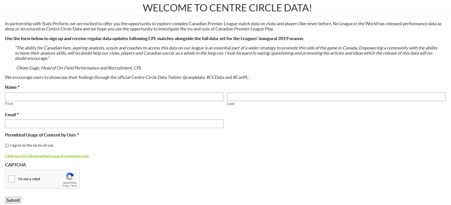
So, it’s nice that we have all this data in a Google Drive folder and that it’s being updated every few days by Centre Circle. However, it’s a bit annoying to have to manually re-download the data files after every update, save it in the proper folder, and only then finally get down to analyzing the data. This is where automation can help, in this case Github Actions and the {googledrive} R package can be utilized to create an ETL pipeline to automate the data loading/saving for you.
Guide
In the following section I’ll go over the steps you need to create an EPL pipeline for CPL data. This tutorial assumes you know the basics of R programming, that you already have a Github account, and can navigate your way around the platform.
It can be a daunting process to set all this up, especially the Google service account stuff. It was the same for me, I had to go through the documentation provided by the {googledrive} R package quite a bit along with a lot of googling things separately.
- {googledrive} R package documentation
- Non-interactive authentication docs from the {gargle} R package
Here is the link to my own
repository, CanPL_Analysis, which has all the files I’ll be talking
about later.
Google Drive
-
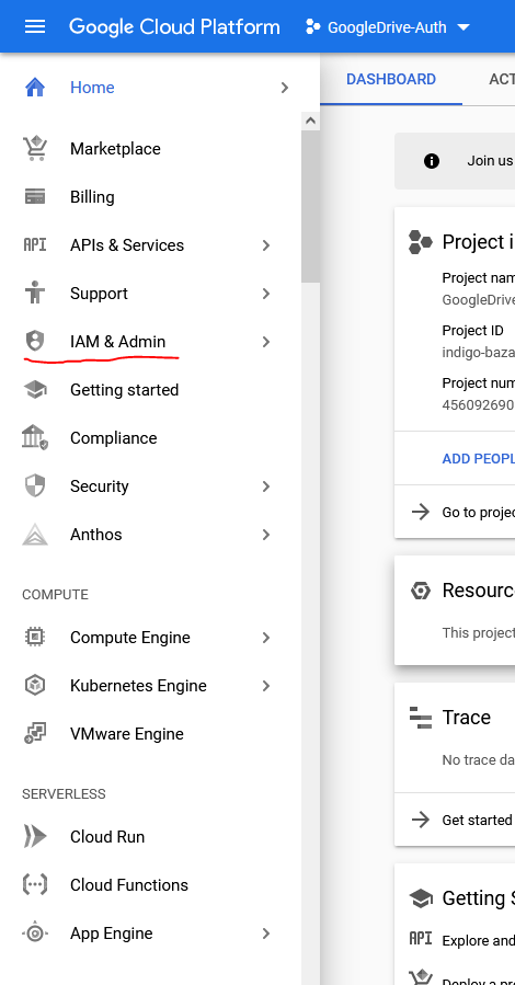
- Make sure you’re already signed into your Google account and go to “Google Cloud Platform/Console”. On the left-side menu bar go to the “IAM & Admin” section.
-
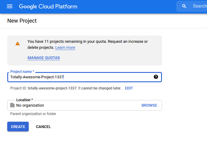
- Scroll down to find the Create a project button in the menu bar. Give it a good name that states the purpose of your project.
-
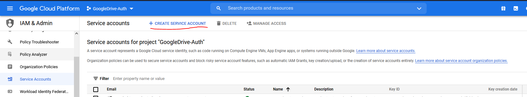
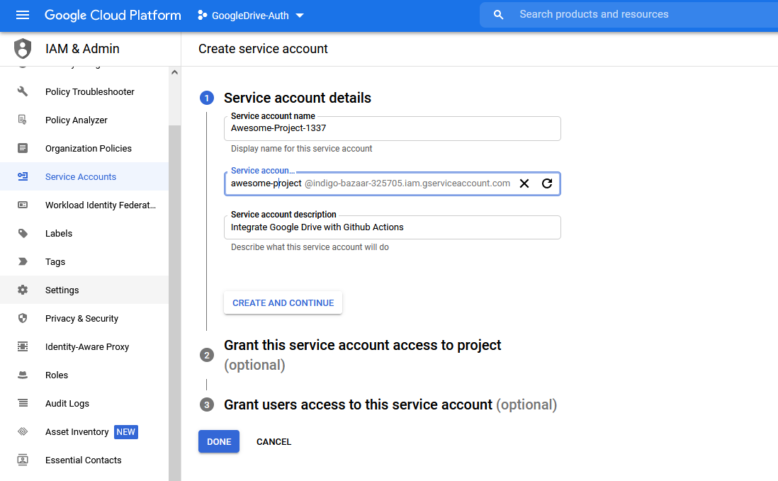
- Create service account. Fill in service account details.
-
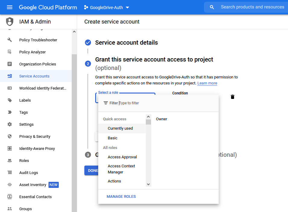
- Select Role “Owner” or other as is relevant for your project.
-
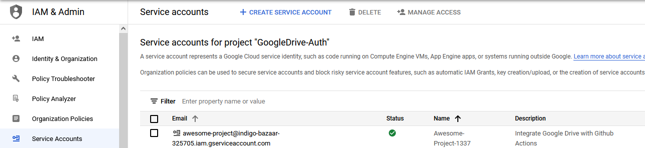
- Once you’re done, click on your newly created service account from the project page. The email you see listed for your service account is something you’ll need later so keep a copy of that address somewhere.
-
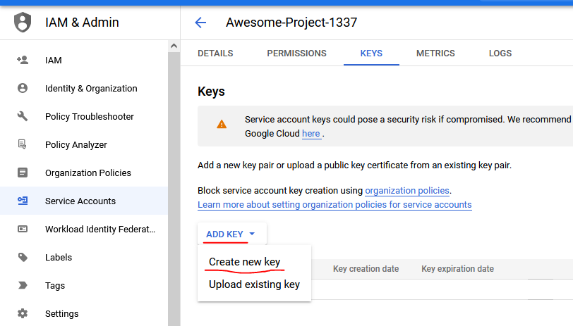
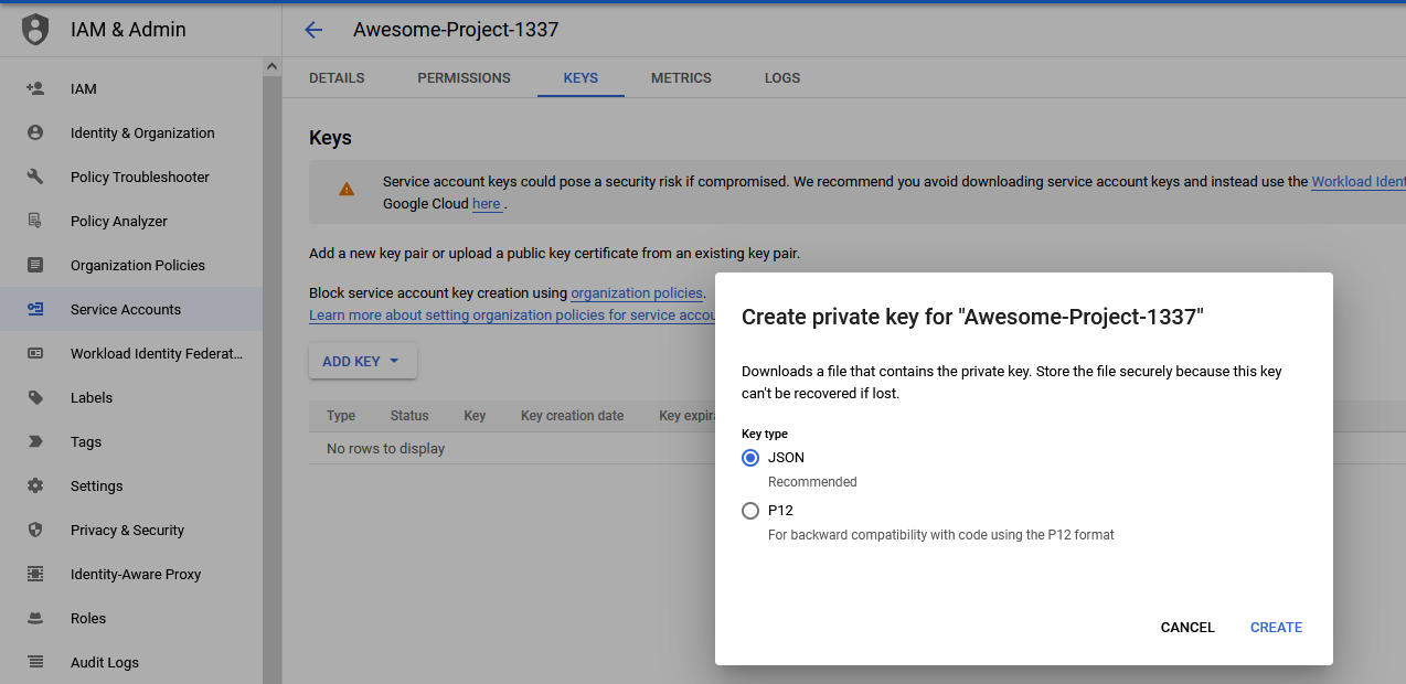
- Go to “Keys” tab and click on “ADD KEY” and then “Create new key”.
-
- Make sure the key type is “JSON” and create it.
-
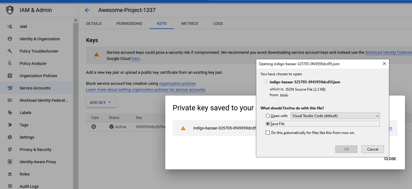
- Store the file in a secure space. Make sure you store it
somewhere so that it’s NOT being uploaded into a public
repository on Github. You can do that by .gitignore-ing the file
or making the credential an environment variable in R with
usethis::edit_r_environ().
- Store the file in a secure space. Make sure you store it
somewhere so that it’s NOT being uploaded into a public
repository on Github. You can do that by .gitignore-ing the file
or making the credential an environment variable in R with
-
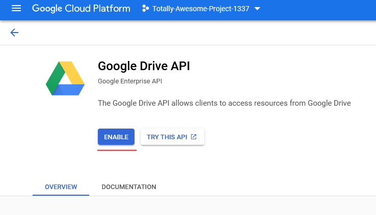
- Go to your Google Drive API page and enable the API. URL link
is:
https://console.developers.google.com/apis/api/drive.googleapis.com/overview?project={YOUR-PROJECT-ID}(fill in {YOUR-PROJECT-ID} with your project ID).
- Go to your Google Drive API page and enable the API. URL link
is:
-
- Ask the owner of folder/file to share it with the service
account by right-clicking on the folder/file in Google Drive and
click the ‘Share’ button (Steven Scott is the owner of CanPL
data). Use the email address you see in the “client_email”
section of your Google credential
JSONfile as the account to add.
- Ask the owner of folder/file to share it with the service
account by right-clicking on the folder/file in Google Drive and
click the ‘Share’ button (Steven Scott is the owner of CanPL
data). Use the email address you see in the “client_email”
section of your Google credential
NOTE: Since the service account doesn’t have a physical email inbox, you can’t send an email to it with the share link and open the file/folder from the email message. You have to make sure to ‘share’/‘ask to share’ the folder/file from Google Drive directly.
NOTE: Please only do this part if you are serious about using the Canadian Premier League data and that you signed up here on the Canadian PL website and have read all the terms, conditions, and “best practices” sheet provided in the Google Drive folder containing the data. Otherwise you can create your own separate folder on Google Drive, put some random data in it, and share that to your Google service account and run the Github Actions workflow on that instead.
Github Actions (GHA)
Github Actions (GHA) is a relatively new feature introduced in late 2019 that allows you to set up workflows and take advantage of Github’s VMs (Windows, Mac, Linux, or your own setup). For using Github Actions with R, there’s a perfectly named Github Actions with R book to help you out, while I have gotten a lot of mileage from looking up other people’s GHA yaml files online and see how they tackled problems. R has considerable support for using Github Actions to power your analyses. Take a look at R-Lib’s GHA repository which will give you templates and commands to set up different workflows for your needs.
Some other examples of using R and GHA:
- Automate Web Scraping in R with Github Actions
- Automating web scraping with GitHub Actions and R: an example from New Jersey
- R-Package GitHub Actions via {usethis} and r-lib
- Up-to-date blog stats in your README
- Launch an R script using github actions (R for SEO book)
- A Twitter bot with {rtweet} and GitHub Actions
To set up GHA in your own Github repository:
-
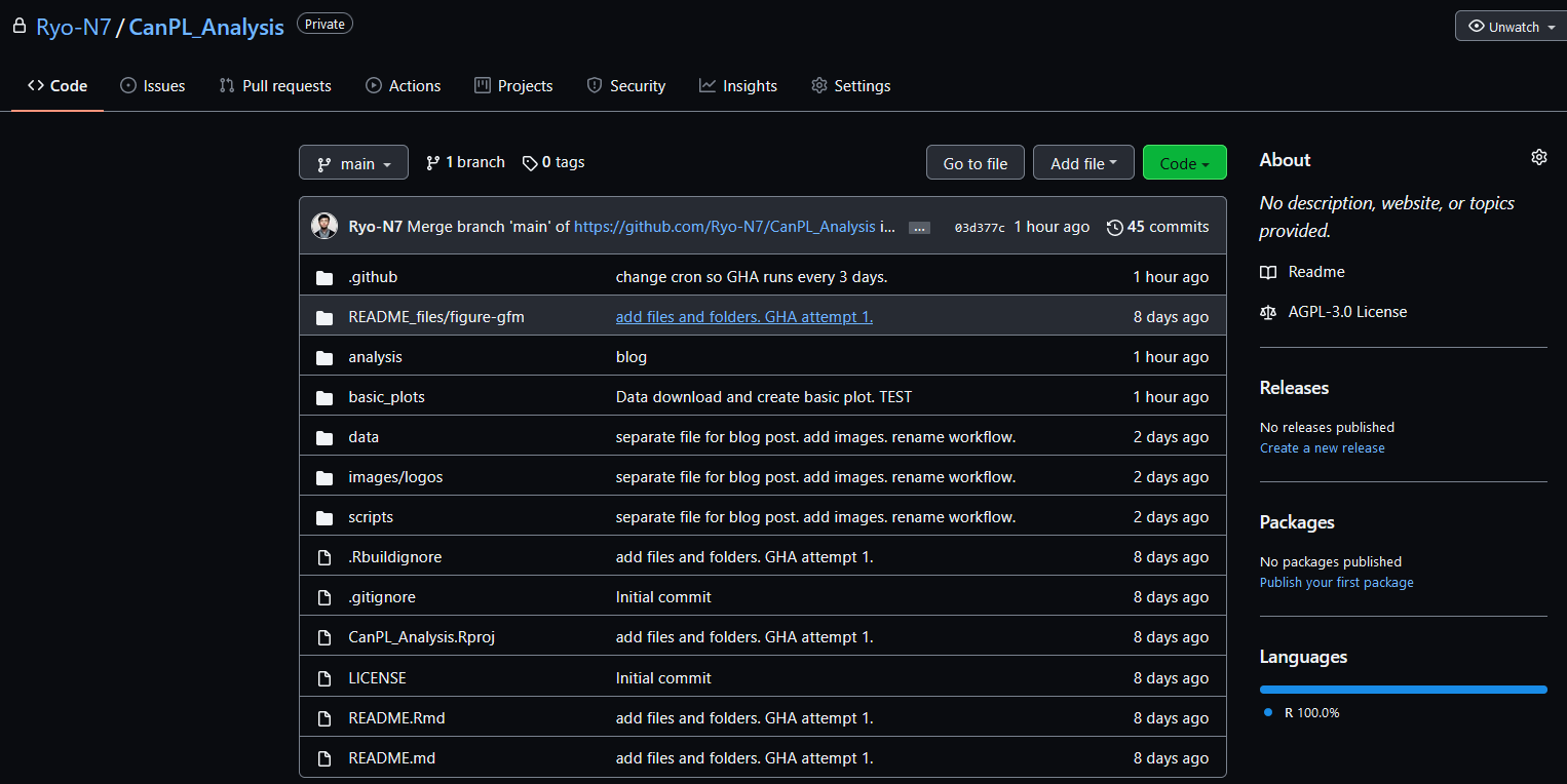
- Have a Github repository set up with the scripts and other materials you want to use. Below is how I set up mine (link), the folders are important as we’re going to be referring to them to save our data and output. Name yours however you wish, just remember to refer to them properly in the R scripts or YAML files you use.
-
- Open the repo up in RStudio and type in:
usethis::use_github_actions(). This will do all the set up for you to get GHA running in your repository.
- Open the repo up in RStudio and type in:
-
- Your GHA workflows are stored in the
.github/workflowsfolder as YAML files. If you used the function above it’ll create one forR-CMD-checkfor you. You don’t need that for what we’re doing since this repository isn’t an R package. Either delete it or modify it for what we want to do. We’ll be working on the YAML files in the next section.
- Your GHA workflows are stored in the
-
- Note that for both private and public repositories you have a number of free credits to use per month but anything more is going to cost you. See here for pricing details.
To let Github Actions workflow use your Google credentials, you need to store it in a place where GHA can retrieve it when its running.
-
- Go into “Settings” in your Github repository, then “Secrets”, and then “New repository secret”.
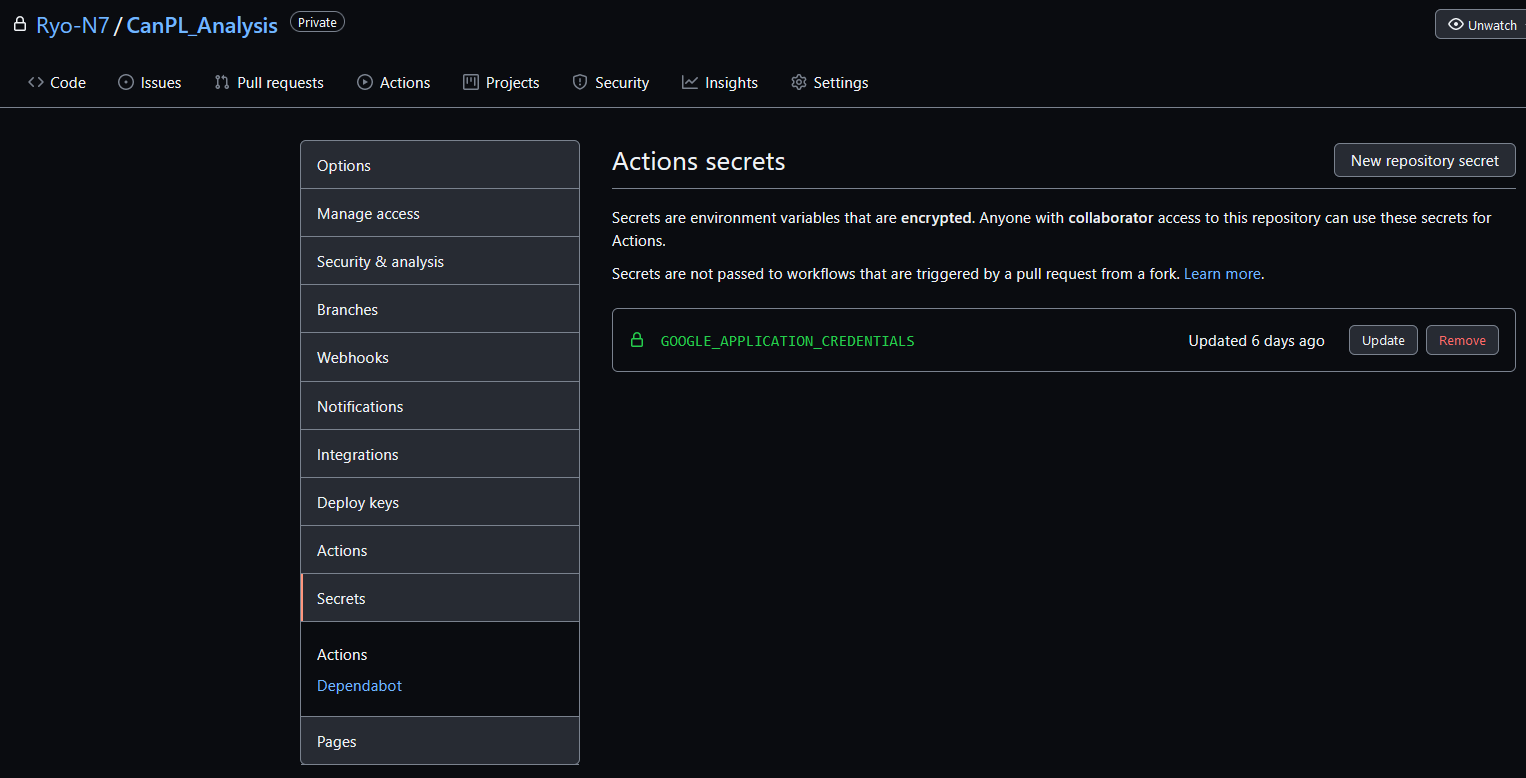
-
- Call it
GOOGLE_AUTHENTICATION_CREDENTIALSor whatever you want (just make sure its consistent between what you call it here and in the workflow YAML file or R script). Then copy-paste the contents of the Google credential key.JSONfile (the one you downloaded earlier) into the “value” prompt. I believe you need to include the{}brackets as well.
- Call it

Workflow YAML file
Now we need to create a workflow YAML file within the
.github/workflows/ directory. This is the file which gives GHA
instructions on what to do. Here is the
link
to the one I created.
First, you want to figure out how often you want this GHA to run. It
really depends on what you want to do with GHA. For the purposes of the
CPL data project, it appears that there are new data updates every few
days so you may want to schedule it to run maybe every two days. It
really depends. To schedule your GHA workflow you can use keywords such
as “push”, “pull-request”, etc. or you can use cron.
The crontab.guru is a useful website to
configure the specific syntax you need to schedule your GHA workflow
with cron, whether that be ‘once a day’, ‘every 3 hours’, ‘every 2
days at 3 AM’, etc. If you still don’t know, try googling “cron run
every 6 hours” or whatever.
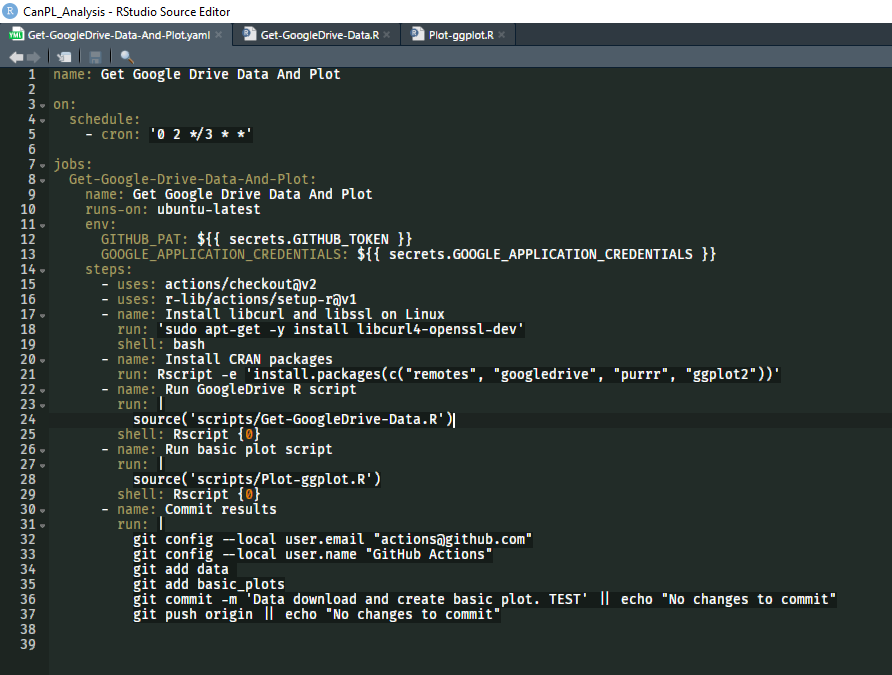
To accomplish what we want to do, the basic steps are as follows:
-
It does some set up with installing R itself (
r-lib/actions/setup-r@v1) and git check out (actions/checkout@v2). -
If you’re using
Ubuntu-Linuxas the VM running this workflow, then you need to installlibcurl opensslto be able to install the {googledrive} package in later steps (mainly due to curl and httr dependency R packages, see this StackOverflow post for details). You don’t need to do this if you’re usingMacOSas the VM. -
Installs R packages from CRAN. Be warned that due to some dependencies, the packages you list here might not actually install even if GHA says that step was completed. This part tripped me up quite a bit until I figured out the
libcurl opensslthing. Also note that there should be a way to cache the R packages you’re installing but so far I’ve only found solutions when the Github repo you’re using is also an R package as well. This part usually takes quite long (and in this simplified example I’m only installing 3 packages!) so if you really want to do something with a lot of dependencies I suggest you research this a lot more or you will use up your GHA minutes quite quickly! -
Runs the R script
Get-GoogleDrive-Data.R. -
Runs the R script
Plot-ggplot.R. -
Commits and pushes the data files downloaded into the Github repository.
Make sure your indentations for each section are correct or it won’t run properly. It can be an annoyance to figure out but it is what it is. I usually just copy-paste someone else’s YAML file that has steps and setups close to what I want to do and then just start editing from there.
More details:
-
on: “When” to run this action. Can be on git push, pull-request, etc. (use[]when specifying multiple conditions) or you can schedule it using cron as we talked about earlier. -
runs-on: Which OS do you want to run this GHA on? Note that per the terms of GHA minutes and billing, using Ubuntu-Linux is the cheapest, then its Windows, and MacOS is the most expensive so plan accordingly. -
env: This is where you refer to the environment variables you have set up in your Github repository. Stuff like your Github Token and your Google service account credentials. -
steps: This is where you outline the specific steps your workflow should take.
An important question is: How can I refer to my Google credentials
stored as a Github secret in the googledrive::drive_auth() function
that will be used in the R script for authentication?
As you specified the Github secret in the previous section as
“GOOGLE_AUTHENTICATION_CREDENTIALS”, you can use that name as the
reference for the Sys.getenv() function so that it can grab that as an
environment variable. You’ll see how that works in the next section.
Also remember that you need to “git pull” your repo whenever so that you have the latest data to work with. This is because when the GHA workflow downloads and commits the data into your github repo, it is only updating it online on github and not on your local computer. So you need to pull all the new stuff in first or you’ll be working with un-updated data from the last time you pulled.
R Scripts
Now that we’ve done a lot of the setup, we can actually start doing
stuff in R. For both of these scripts I tried using the minimal amount
of packages to reduce dependencies that GHA would have to download and
install as part of the workflow run. You could easily use a for loop
instead of purrr::map2() and base R plotting instead of {ggplot2} if
you want to go even further (I attempted this in scripts/Plot-BaseR.R
but it was just quicker doing it with ggplot2).
Get-GoogleDrive-Data.R
-
Load R packages.
-
Authenticate Google Drive by fetching the environment variable you set up in the Github repository as a Github secret.
-
Find the Google Drive folder you want to grab data from.
-
Filter the folder for the
.csvfiles. -
Create a download function that grabs the
.csvfiles and saves them in thedata/folder. Add some handy messages throughout the function so that it will show up in the GHA log (this helps with debugging and just knowing what’s going on as the workflow runs). -
Now use
purrr::map2()to iterate the download function to each individual.csvfile in the folder.
## Load packages ----
library(googledrive)
library(purrr)
#library(dplyr)
#library(stringr)
#library(fs)
options(googledrive_quiet = TRUE)

## Authenticate into googledrive service account ----
## 'GOOGLE_APPLICATION_CREDENTIALS' is what we named the Github Secret that
## contains the credential JSON file
googledrive::drive_auth(path = Sys.getenv("GOOGLE_APPLICATION_CREDENTIALS"))

## Find Google Drive folder 'Centre Circle Data & Info'
data_folder <- drive_ls(path = "Centre Circle Data & Info")

## Filter for just the .csv files
data_csv <- data_folder[grepl(".csv", data_folder$name), ]
# dplyr: data_csv <- data_folder %>% filter(str_detect(name, ".csv")) %>% arrange(name)

data_path <- "data"
dir.create(data_path)
## dir.create will fail if folder already exists so not great for scripts on local but as GHA is
## creating a new environment every time it runs we won't have that problem here
# normally i prefer using fs::dir_create(data_path)

## download function ----
get_drive_cpl_data <- function(g_id, data_name) {
  cat("\n... Trying to download", data_name, "...\n")

  # Wrap drive_download function in safely()
  safe_drive_download <- purrr::safely(drive_download)

  ## Run download function for all data files
  dl_return <- safe_drive_download(file = as_id(g_id), path = paste0("data/", data_name), overwrite = TRUE)

  ## Log messages for success or failure
  if (is.null(dl_return$result)) {
    cat("\nSomething went wrong!\n")
    dl_error <- as.character(dl_return$error) ## errors come back as lists sometimes so coerce to character
    cat("\n", dl_error, "\n")
  } else {
    res <- dl_return$result
    cat("\nFile:", res$name, "download successful!", "\nPath:", res$local_path, "\n")
  }
}

## Download all files from Google Drive! ----
map2(data_csv$id, data_csv$name,
     ~ get_drive_cpl_data(g_id = .x, data_name = .y))

cat("\nAll done!\n")
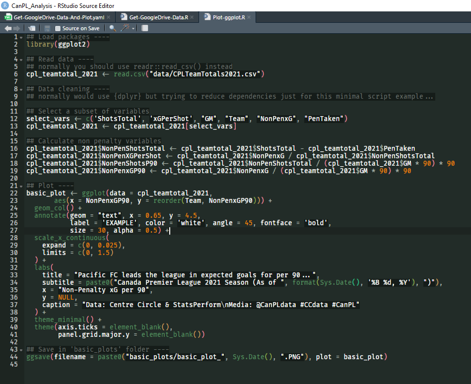
Plot-ggplot.R
-
Load R packages.
-
Read data from the
data/folder. -
Do some data cleaning and create some non-penalty version of the variables.
-
Create a very basic bar chart.
-
Save it in the
basic_plots/folder.
## Load packages ----
library(ggplot2)

## Read data ----
## normally you should use readr::read_csv() instead
cpl_teamtotal_2021 <- read.csv("data/CPLTeamTotals2021.csv")

## Data cleaning ----
## normally would use {dplyr} but trying to reduce dependencies just for this minimal script example...

## Select a subset of variables
select_vars <- c('ShotsTotal', 'xGPerShot', "GM", "Team", "NonPenxG", "PenTaken")
cpl_teamtotal_2021 <- cpl_teamtotal_2021[select_vars]

## Calculate non penalty variables
cpl_teamtotal_2021$NonPenShotsTotal <- cpl_teamtotal_2021$ShotsTotal - cpl_teamtotal_2021$PenTaken
cpl_teamtotal_2021$NonPenXGPerShot <- cpl_teamtotal_2021$NonPenxG / cpl_teamtotal_2021$NonPenShotsTotal
cpl_teamtotal_2021$NonPenShotsP90 <- cpl_teamtotal_2021$NonPenShotsTotal / (cpl_teamtotal_2021$GM * 90) * 90
cpl_teamtotal_2021$NonPenxGP90 <- cpl_teamtotal_2021$NonPenxG / (cpl_teamtotal_2021$GM * 90) * 90

## Plot ----
basic_plot <- ggplot(data = cpl_teamtotal_2021,
       aes(x = NonPenxGP90, y = reorder(Team, NonPenxGP90))) +
  geom_col() +
  annotate(geom = "text", x = 0.65, y = 4.5,
           label = 'EXAMPLE', color = 'white', angle = 45, fontface = 'bold',
           size = 30, alpha = 0.5) +
  scale_x_continuous(
    expand = c(0, 0.025),
    limits = c(0, 1.5)
  ) +
  labs(
    title = "Pacific FC leads the league in expected goals for per 90...",
    subtitle = paste0("Canada Premier League 2021 Season (As of ", format(Sys.Date(), '%B %d, %Y'), ")"),
    x = "Non-Penalty xG per 90",
    y = NULL,
    caption = "Data: Centre Circle & StatsPerform\nMedia: @CanPLdata #CCdata #CanPL"
  ) +
  theme_minimal() +
  theme(axis.ticks = element_blank(),
        panel.grid.major.y = element_blank())

## Save in 'basic_plots' folder ----
ggsave(filename = paste0("basic_plots/basic_plot_", Sys.Date(), ".PNG"), plot = basic_plot)
Output
Once a workflow is successful, you should be able to see that another
git commit was made in your github repository that saved new data
downloaded from the CanPL Google Drive folder into your data/ folder,
while the simple plot of xG data was saved and committed in the
basic_plots folder. When you’re creating work from this data set
please remember to add in social media links to the Canadian Premier
League as well as the logos for Centre Circle Data and StatsPerform
(below example plot is without the logos).
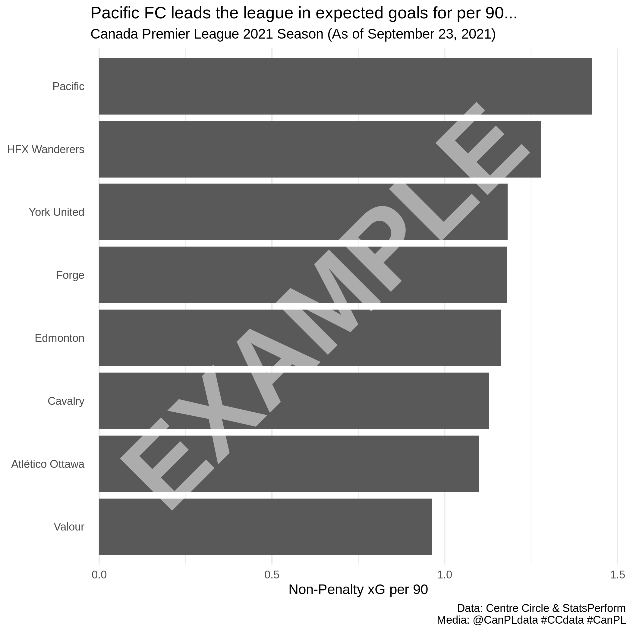
(It’s very possible that as the data is updated throughout the season, Pacific FC won’t be the league leaders but whatever, you get the point.)
Conclusion
Hopefully this was a helpful guide for grabbing Canadian Premier League soccer data automatically with Github Actions. There is a lot to learn as there are many different moving parts to make this work. I tried to put links to a lot of the documentation and blog posts that helped me through so those should be of use to you as well.
There are many things you can do by extending the very basic ETL set up we created in this blog post, including but not limited to:
- Create a Twitter bot to post your visualizations!
- Create a parameterized RMarkdown report!
- Create a Rmarkdown dashboard!
- Use the updated data to power a Shiny app!
- Create your own separate database and upload new data into it after some cleaning steps!
- Etc.
Some of these are things which I hope to talk about in future blog posts, so stay tuned!