Another year, another big soccer/football tournament! This time it’s the
top international competition in Asia, the Asian Cup hosted in the
U.A.E. In this blog post I’ll be covering (responsible) web-scraping, data wrangling
(tidyverse FTW!), and of course, data visualization with ggplot2. All of the code and data below is also uploaded in my soccer_ggplots Github repo.
Let’s get started!
Packages
pacman::p_load(tidyverse, scales, lubridate, ggrepel, stringi, magick,
               glue, extrafont, rvest, ggtextures, cowplot, ggimage, polite)
# Roboto Condensed font (from hrbrmstrthemes)
loadfonts()
Top Goalscorers of the Asian Cup
The first thing I looked at was, “Who are the top goalscorers in the history of the Asian Cup?”
Here I use the polite package to
take a look at the robots.txt for the web page and see if it is OK to
web scrape from it. First you pass the URL to the bow() function, check that you are
indeed allowed to scrape, then use scrape() to retrieve data, and the
rest is the usual rvest web-scraping workflow.
topg_url <- "https://en.wikipedia.org/wiki/AFC_Asian_Cup_records_and_statistics"

session <- bow(topg_url)

ac_top_scorers <- scrape(session) %>%
  html_nodes("table.wikitable:nth-child(29)") %>%
  html_table() %>%
  flatten_df() %>%
  select(-Ref.) %>%
  set_names(c("total_goals", "player", "country"))
For brevity, let’s only take a look at the top 5 goal scorers. I’ll also
mutate() in a nice image of a soccer ball for the data points on the
plot.
ac_top_scorers <- ac_top_scorers %>%
  head(5) %>%
  mutate(image = "https://www.emoji.co.uk/files/microsoft-emojis/activity-windows10/8356-soccer-ball.png")
I made something slightly different to your standard bar graph as I
use the geom_isotype_col() function from ggtextures to create a bar
of soccer ball images. Compared to other functions in ggtextures,
geom_isotype_col() allows each image to correspond to the value of the
variable you are plotting, in this case 1 ball = 1 goal!
ac_top_graph <- ac_top_scorers %>%
  ggplot(aes(x = reorder(player, total_goals), y = total_goals,
             image = image)) +
  geom_isotype_col(img_width = grid::unit(1, "native"), img_height = NULL,
    ncol = NA, nrow = 1, hjust = 0, vjust = 0.5) +
  coord_flip() +
  scale_y_continuous(breaks = c(0, 2, 4, 6, 8, 10, 12, 14),
                     expand = c(0, 0),
                     limits = c(0, 15)) +
  ggthemes::theme_solarized() +
  labs(title = "Top Scorers of the Asian Cup",
       subtitle = "Most goals in a single tournament: 8 (Ali Daei, 1996)",
       y = "Number of Goals", x = NULL,
       caption = glue("
                      Source: Wikipedia
                      By @R_by_Ryo")) +
  theme(text = element_text(family = "Roboto Condensed"),
        plot.title = element_text(size = 22),
        plot.subtitle = element_text(size = 14),
        axis.text = element_text(size = 14),
        axis.title.x = element_text(size = 16),
        axis.line.y = element_blank(),
        panel.grid.minor = element_blank(),
        panel.background = element_blank(),
        axis.ticks.y = element_blank())

ac_top_graph
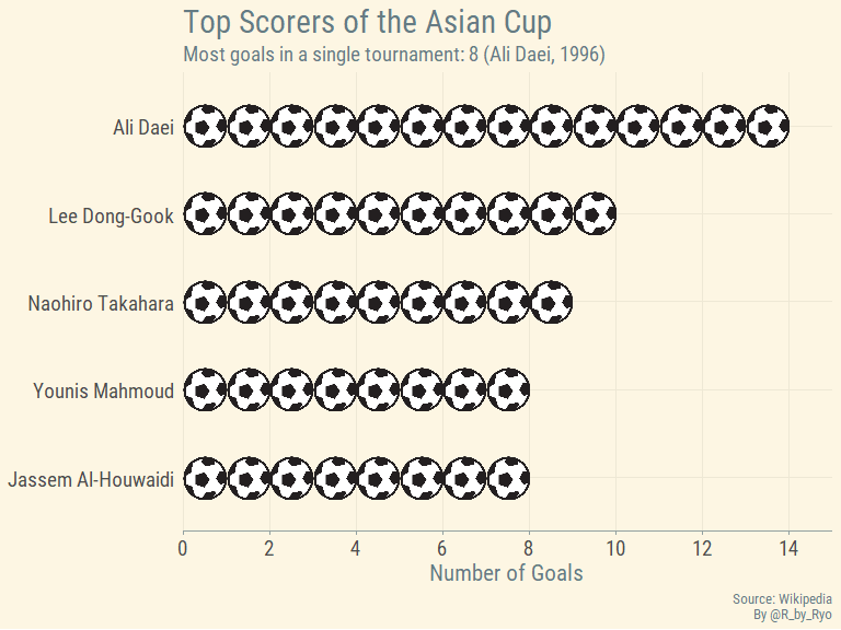
OK, not bad. However, wouldn’t it be nice to add a bit more context? Specifically, which country these players came from. So let’s add some flags along the y-axis!
There are lots of different ways to do this (like geom_flag() from the
ggimage package) but I ended up doing it the cowplot way. I had to
tweak the scales a bit as the flags came in different sizes. When you
plot, you just insert the image strip into the bar plot with
axis_canvas() and combine all the parts together with ggdraw()!
axis_image <- axis_canvas(ac_top_graph, axis = 'y') +
  draw_image("https://upload.wikimedia.org/wikipedia/commons/c/ca/Flag_of_Iran.svg",
             y = 13, scale = 1.5) +
  draw_image("https://upload.wikimedia.org/wikipedia/commons/0/09/Flag_of_South_Korea.svg",
             y = 10, scale = 1.7) +
  draw_image("https://upload.wikimedia.org/wikipedia/en/9/9e/Flag_of_Japan.svg",
             y = 7, scale = 1.7) +
  draw_image("https://upload.wikimedia.org/wikipedia/commons/f/f6/Flag_of_Iraq.svg",
             y = 4, scale = 1.6) +
  draw_image("https://upload.wikimedia.org/wikipedia/commons/a/aa/Flag_of_Kuwait.svg",
             y = 1, scale = 1.2)

ggdraw(insert_yaxis_grob(ac_top_graph, axis_image, position = "left"))
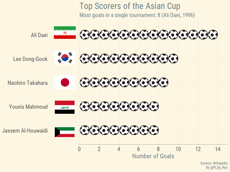
Ideally I wanted the soccer balls to be the official balls from the tournament that the player scored in. However, I couldn’t find a nice emoji-fied/icon-ized version and there was also the “small” problem in that there was no “official” Asian Cup ball until the 2004 tournament in China! You can take a look at the official Asian Cup balls here.
Winners of the Asian Cup
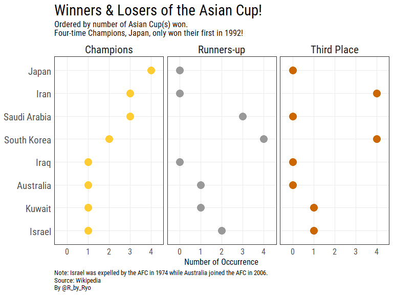
We saw that the top goal scorers came from Iran, South Korea, Japan, Iraq, and Kuwait but did their goal scoring exploits lead their nations to glory? Let’s find out!
When web-scraping I really like using flatten_df() after
html_table() as I don’t have to use the awkward looking .[[1]]
within my piped workflow.
acup_url <- "https://en.wikipedia.org/wiki/AFC_Asian_Cup"

session <- bow(acup_url)

acup_winners_raw <- scrape(session) %>%
  html_nodes("table:nth-child(31)") %>%
  html_table() %>%
  flatten_df()
Now I can use the clean_names() function to quickly clean up my column names
(mainly when I can’t be bothered to set_names() them myself…).
The next steps are splitting up the number of times a team placed
between 1st and 3rd and the year that occurred with separate(). Then variants of mutate() are used to tidy the string columns of the data into numeric type. I use gather() so each team will have a row for each of the rank positions (1st-3rd). Finally, I arrange the data in a way that the facets will be ordered in the way that I want.
acup_winners_clean <- acup_winners_raw %>%
  janitor::clean_names() %>%
  slice(1:8) %>%
  select(-fourth_place, -semi_finalists, -total_top_four) %>%
  separate(winners, into = c("Champions", "first_place_year"),
           sep = " ", extra = "merge") %>%
  separate(runners_up, into = c("Runners-up", "second_place_year"),
           sep = " ", extra = "merge") %>%
  separate(third_place, into = c("Third Place", "third_place_year"),
           sep = " ", extra = "merge") %>%
  mutate_all(funs(str_replace_all(., "–", "0"))) %>%
  mutate_at(vars(contains("num")), funs(as.numeric)) %>%
  mutate(team = if_else(team == "Israel1", "Israel", team)) %>%
  gather(key = "key", value = "value", -team,
         -first_place_year, -second_place_year, -third_place_year) %>%
  mutate(key = key %>%
           fct_relevel(c("Champions", "Runners-up", "Third Place"))) %>%
  arrange(key, value) %>%
  mutate(team = as_factor(team),
         order = row_number())
I plot using facets on the “key” variable (containing the rank data) so
that we can see how many times each team placed as Champions to Third
Place. I also use the glue() function here to format the multi-line
captions and titles in a neat way.
acup_winners_clean %>%
  ggplot(aes(value, team, color = key)) +
  geom_point(size = 5) +
  scale_color_manual(values = c("Champions" = "#FFCC33",
                                "Runners-up" = "#999999",
                                "Third Place" = "#CC6600"),
                     guide = FALSE) +
  labs(x = "Number of Occurrence",
       title = "Winners & Losers of the Asian Cup!",
       subtitle = glue("
                       Ordered by number of Asian Cup(s) won.
                       Four-time Champions, Japan, only won their first in 1992!"),
       caption = glue("
                      Note: Israel was expelled by the AFC in 1974 while Australia joined the AFC in 2006.
                      Source: Wikipedia
                      By @R_by_Ryo")) +
  facet_wrap(~key) +
  theme_minimal() +
  theme(text = element_text(family = "Roboto Condensed"),
        title = element_text(size = 18),
        plot.subtitle = element_text(size = 12),
        axis.title.y = element_blank(),
        axis.title.x = element_text(size = 12),
        axis.text.y = element_text(size = 14),
        axis.text.x = element_text(size = 12),
        plot.caption = element_text(hjust = 0, size = 10),
        panel.border = element_rect(fill = NA, colour = "grey20"),
        panel.grid.minor.x = element_blank(),
        strip.text = element_text(size = 16))
Goals per Game
One new thing I learned very recently, while working on this viz in
fact, was using magrittr aliases! In this workflow I always wind up having to use .[x] or
.[[x]] but now I can just use extract() or extract2() respectively
to do the same thing!
wiki_url <- "https://en.wikipedia.org"
session <- bow(wiki_url)
acup_url <- "https://en.wikipedia.org/wiki/AFC_Asian_Cup"
session_cup <- bow(acup_url)

cup_links <- scrape(session_cup) %>%
  html_nodes("br+ i a") %>%
  html_attr("href") %>%
  magrittr::extract(-17:-18)

acup_df <- cup_links %>%
  as_data_frame() %>%
  mutate(cup = str_remove(value, "\\/wiki\\/") %>% str_replace_all("_", " ")) %>%
  rename(link = value)
Another cool thing I found while scraping this data was the jump_to()
function that allows you to navigate to a new URL. This makes
map()-ing over multiple URL links from a base URL very easy! Here, the
base URL is the AFC Asian Cup Wikipedia page and the function iterates
over each of the URL links of the respective tournament pages.
Another way that I could’ve done this was to map() over the different
dates of the tournaments as the Wikipedia page of each edition of the
Asian Cup only differed in the “year” appended at the beginning of the
URL.
goals_info <- function(x) {
  goal_info <- scrape(session) %>%
    jump_to(x) %>%
    html_nodes(".vcalendar") %>%
    html_table(header = FALSE) %>%
    flatten_df() %>%
    spread(key = X1, value = X2) %>%
    select(`Goals scored`) %>%
    mutate(`Goals scored` = str_remove_all(`Goals scored`, pattern = ".*\\(") %>%
             str_extract_all("\\d+\\.*\\d*") %>% as.numeric)
}

team_num_info <- function(x) {
  team_num_info <- scrape(session) %>%
    jump_to(x) %>%
    html_nodes(".vcalendar") %>%
    html_table(header = FALSE) %>%
    flatten_df() %>%
    spread(key = X1, value = X2) %>%
    select(`Teams`) %>%
    mutate(`Teams` = as.numeric(`Teams`))
}

match_num_info <- function(x) {
  match_num_info <- scrape(session) %>%
    jump_to(x) %>%
    html_nodes(".vcalendar") %>%
    html_table(header = FALSE) %>%
    flatten_df() %>%
    spread(key = X1, value = X2) %>%
    janitor::clean_names() %>%
    select(matches_played) %>%
    mutate(matches_played = as.numeric(matches_played))
}

# all together:
goals_data <- acup_df %>%
  mutate(goals_per_game = map(acup_df$link, goals_info) %>% unlist,
         team_num = map(acup_df$link, team_num_info) %>% unlist,
         match_num = map(acup_df$link, match_num_info) %>% unlist)
Next, I clean it up a bit and add in the number of teams that participated in each tournament.
ac_goals_df <- goals_data %>%
  mutate(label = cup %>% str_extract("[0-9]+") %>% str_replace("..", "'"),
         team_num = case_when(
           is.na(team_num) ~ 16,
           TRUE ~ team_num
         )) %>%
  arrange(cup) %>%
  mutate(label = factor(label, label),
         team_num = c(4, 4, 4, 5, 6, 6, 10, 10, 10, 8, 12, 12, 16, 16, 16, 16))

glimpse(ac_goals_df)
## Observations: 16
## Variables: 6
## $ link           <chr> "/wiki/1956_AFC_Asian_Cup", "/wiki/1960_AFC_Asi...
## $ cup            <chr> "1956 AFC Asian Cup", "1960 AFC Asian Cup", "19...
## $ goals_per_game <dbl> 4.50, 3.17, 2.17, 3.20, 2.92, 2.50, 3.17, 1.83,...
## $ team_num       <dbl> 4, 4, 4, 5, 6, 6, 10, 10, 10, 8, 12, 12, 16, 16...
## $ match_num      <dbl> 6, 6, 6, 10, 13, 10, 24, 24, 24, 16, 26, 26, 32...
## $ label          <fct> '56, '60, '64, '68, '72, '76, '80, '84, '88, '9...
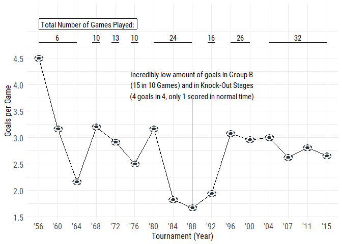
Now we make a line graph but with lots of annotate() code to add in
comments, labels, and segments for the labels. At the end I use
geom_emoji() to add a soccer ball to the plot for each of the data
points.
plot <- ac_goals_df %>%
  ggplot(aes(x = label, y = goals_per_game, group = 1)) +
  geom_line() +
  scale_y_continuous(limits = c(NA, 5.35),
                     breaks = c(1.5, 2, 2.5, 3, 3.5, 4, 4.5)) +
  labs(x = "Tournament (Year)", y = "Goals per Game") +
  theme_minimal() +
  theme(text = element_text(family = "Roboto Condensed"),
        axis.title = element_text(size = 12),
        axis.text = element_text(size = 12)) +
  annotate(geom = "label", x = "'56", y = 5.15, family = "Roboto Condensed",
           color = "black",
           label = "Total Number of Games Played:", hjust = 0) +
  annotate(geom = "text", x = "'60", y = 4.9,
           label = "6", family = "Roboto Condensed") +
  annotate(geom = "segment", x = 1, xend = 3, y = 4.8, yend = 4.8) +
  annotate(geom = "text", x = "'68", y = 4.9,
           label = "10", family = "Roboto Condensed") +
  annotate(geom = "segment", x = 3.8, xend = 4.2, y = 4.8, yend = 4.8) +
  annotate(geom = "text", x = "'72", y = 4.9,
           label = "13", family = "Roboto Condensed") +
  annotate(geom = "segment", x = 4.8, xend = 5.2, y = 4.8, yend = 4.8) +
  annotate(geom = "text", x = "'76", y = 4.9,
           label = "10", family = "Roboto Condensed") +
  annotate(geom = "segment", x = 5.8, xend = 6.2, y = 4.8, yend = 4.8) +
  annotate(geom = "text", x = "'84", y = 4.9,
           label = "24", family = "Roboto Condensed") +
  annotate(geom = "segment", x = 7, xend = 9, y = 4.8, yend = 4.8) +
  annotate(geom = "text", x = "'92", y = 4.9,
           label = "16", family = "Roboto Condensed") +
  annotate(geom = "segment", x = 9.8, xend = 10.2, y = 4.8, yend = 4.8) +
  annotate(geom = "text", x = 11.5, y = 4.9,
           label = "26", family = "Roboto Condensed") +
  annotate(geom = "segment", x = 11, xend = 12, y = 4.8, yend = 4.8) +
  annotate(geom = "text", x = 14.5, y = 4.9,
           label = "32", family = "Roboto Condensed") +
  annotate(geom = "segment", x = 13, xend = 16, y = 4.8, yend = 4.8) +
  annotate(geom = "text", x = 9, y = 4, family = "Roboto Condensed",
           label = glue("
                        Incredibly low amount of goals in Group B
                        (15 in 10 Games) and in Knock-Out Stages
                        (4 goals in 4, only 1 scored in normal time)")) +
  annotate(geom = "segment", x = 9, xend = 9, y = 1.65, yend = 3.75,
           color = "red") +
  ggimage::geom_emoji(aes(image = '26bd'), size = 0.03)

plot
ggsave(filename = glue("{here::here('Asian Cup 2019')}/gpg_plot_final.png"),
       width = 8, height = 7, dpi = 300)
plot <- image_read(glue("{here::here('Asian Cup 2019')}/gpg_plot_final.png"))
However, I’m not finished yet! I wanted to try to make this look a bit
more “official” so I attempted to add the Asian Cup logo on the top
right corner. There are probably alternative ways to how I did it below,
especially by using grobs, but I was reminded of
this blog post by Daniel
Hadley who used the magick package
to add a footer with a logo onto a ggplot object. I’ve used magick
before for animations and this was a good chance to try it out for image
editing. Compared to Daniel Hadley’s example I needed to have the logo
on the right corner so I had to create a blank canvas with image_blank() and then placing everything on top of that with image_composite() and image_append().
logo_raw <- image_read("https://upload.wikimedia.org/wikipedia/en/a/ad/2019_afc_asian_cup_logo.png")

logo_proc <- logo_raw %>% image_scale("600")

# create blank canvas
a <- image_blank(width = 1000, height = 100, color = "white")
# combine with logo image and shift logo to the right
b <- image_composite(image_scale(a, "x100"), image_scale(logo_proc, "x75"),
                     offset = "+880+25")
# add in the title text
logo_header <- b %>%
  image_annotate(text = glue("Goals per Game Throughout the History of the Asian Cup"),
                 color = "black", size = 24, font = "Roboto Condensed",
                 location = "+63+50", gravity = "northwest")

# combine it all together!
final2_plot <- image_append(image_scale(c(logo_header, plot), "1000"), stack = TRUE)

# image_write(final2_plot,
#             glue("{here::here('Asian Cup 2019')}/gpg_plot_final.png"))

final2_plot
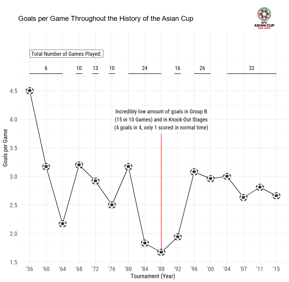
All in all it took a while to tweak the positions of the text and logo image but for my first try it worked well. There is definitely room for improvement in regards to sizing and scaling though.
Ultimately, I couldn’t find much information on why those tournaments in the 80s in particular were such low scoring affairs. I wasn’t alive to watch those games on TV nor could I find any illuminating articles or blog posts on the style of Asian football back then… This was also before Japan really got into soccer so there wasn’t anything I could find in Japanese either.
Japan’s Record vs. Historical Rivals and Group F Opponents
Japan is the most successful team in the competition with 4 championships but who are their opponents in the group stages and how have they fared against them in the past? While I’m at it I will also check Japan’s records against long-time continental rivals such as Iran, South Korea, Saudi Arabia and more recently, Australia.
The data I’m going to use comes from Kaggle which has all international football results from 1872 to the World Cup final last year. To add in the federation affiliation (UEFA, AFC, etc.) for each of the countries I slightly modified some code from one of the kernels, “A Journey Through The History of Soccer” by PH Julien.
federation_files <- Sys.glob("../data/federation_affiliations/*")

df_federations = data.frame(country = NULL, federation = NULL)
for (f in federation_files) {
    federation = basename(f)
    content = read.csv(f, header=FALSE)
    content <- cbind(content,federation=rep(federation, dim(content)[1]))
    df_federations <- rbind(df_federations, content)
}

colnames(df_federations) <- c("country", "federation")

df_federations <- df_federations %>%
  mutate(country = as.character(country) %>% str_trim(side = "both"))
Now to load the results data and then join it with the affiliations data.
results_raw <- read_csv("../data/results.csv")

results_japan_raw <- results_raw %>%
  filter(home_team == "Japan" | away_team == "Japan") %>%
  rename(venue_country = country,
         venue_city = city) %>%
  mutate(match_num = row_number())

# combine with federation affiliations
results_japan_home <- results_japan_raw %>%
  left_join(df_federations,
            by = c("home_team" = "country")) %>%
  mutate(federation = as.character(federation)) %>%
  rename(home_federation = federation)

results_japan_away <- results_japan_raw %>%
  left_join(df_federations,
            by = c("away_team" = "country")) %>%
  mutate(federation = as.character(federation)) %>%
  rename(away_federation = federation)

# combine home-away
results_japan_cleaned <- results_japan_home %>%
  full_join(results_japan_away)
Next I need to edit some of the continents for teams that didn’t have a match in the federation affiliation data set, for example, “South Korea” is “Korea Republic” in the Kaggle data set.
results_japan_cleaned <- results_japan_cleaned %>%
  mutate(
    home_federation = case_when(
      home_team %in% c(
        "China", "Manchukuo", "Burma", "Korea Republic", "Vietnam Republic",
        "Korea DPR", "Brunei") ~ "AFC",
      home_team == "USA" ~ "Concacaf",
      home_team == "Bosnia-Herzegovina" ~ "UEFA",
      TRUE ~ home_federation),
    away_federation = case_when(
      away_team %in% c(
        "China", "Manchukuo", "Burma", "Korea Republic", "Vietnam Republic",
        "Korea DPR", "Brunei", "Taiwan") ~ "AFC",
      away_team == "USA" ~ "Concacaf",
      away_team == "Bosnia-Herzegovina" ~ "UEFA",
      TRUE ~ away_federation
    ))
Now that it’s nice and cleaned up I can reshape it so that the data is set from Japan’s perspective.
results_jp_asia <- results_japan_cleaned %>%
  # filter only for Japan games and AFC opponents
  filter(home_team == "Japan" | away_team == "Japan",
         home_federation == "AFC" & away_federation == "AFC") %>%
  select(-contains("federation"), -contains("venue"),
         -neutral, -match_num,
         date, home_team, home_score, away_team, away_score, tournament) %>%
  # reshape columns to Japan vs. opponent
  mutate(
    opponent = case_when(
      away_team != "Japan" ~ away_team,
      home_team != "Japan" ~ home_team),
    home_away = case_when(
      home_team == "Japan" ~ "home",
      away_team == "Japan" ~ "away"),
    japan_goals = case_when(
      home_team == "Japan" ~ home_score,
      away_team == "Japan" ~ away_score),
    opp_goals = case_when(
      home_team != "Japan" ~ home_score,
      away_team != "Japan" ~ away_score)) %>%
  # label results from Japan's perspective
  mutate(
    result = case_when(
      japan_goals > opp_goals ~ "Win",
      japan_goals < opp_goals ~ "Loss",
      japan_goals == opp_goals ~ "Draw"),
    result = result %>% as_factor() %>% fct_relevel(c("Win", "Draw", "Loss"))) %>%
  select(-contains("score"), -contains("team"))
With all that done we can take a look at how Japan have done against
certain opponents by using filter().
results_jp_asia %>%
  filter(opponent == "Jordan",
         tournament == "AFC Asian Cup")
## # A tibble: 3 x 7
##   date       tournament    opponent home_away japan_goals opp_goals result
##   <date>     <chr>         <chr>    <chr>           <int>     <int> <fct>
## 1 2004-07-31 AFC Asian Cup Jordan   home                1         1 Draw
## 2 2011-01-09 AFC Asian Cup Jordan   home                1         1 Draw
## 3 2015-01-20 AFC Asian Cup Jordan   home                2         0 Win
Unfortunately, this data set doesn’t go into extra-time or penalty wins as Japan’s Quarter-Final meeting with Jordan in 2004 ended with Japan securing a route to the semis, 4-3 on penalties!
I can create a function that’ll filter for certain opponents and
tournaments and aggregate the results. With the second argument being
..., tidyeval allows me to input any kind of filter condition for an
opponent, tournament, etc. The if else statement protects against
cases where Japan never had that type of result against an opponent and
makes sure that a column populated by 0s is created.
japan_versus <- function(data, ...) {
  # filter
  filter_vars <- enquos(...)

  jp_vs <- data %>%
    filter(!!!filter_vars) %>%
    # count results type per opponent
    group_by(result, opponent) %>%
    mutate(n = n()) %>%
    ungroup() %>%
    # sum amount of goals by Japan and opponent
    group_by(result, opponent) %>%
    summarize(j_g = sum(japan_goals),
              o_g = sum(opp_goals),
              n = n()) %>%
    ungroup() %>%
    # spread results over multiple columns
    spread(result, n) %>%
    # 1. failsafe against no type of result against an opponent
    # 2. sum up counts per opponent
    group_by(opponent) %>%
    mutate(Win = if("Win" %in% names(.)){return(Win)} else{return(0)},
         Draw = if("Draw" %in% names(.)){return(Draw)} else{return(0)},
         Loss = if("Loss" %in% names(.)){return(Loss)} else{return(0)}) %>%
    summarize(Win = sum(Win, na.rm = TRUE),
              Draw = sum(Draw, na.rm = TRUE),
              Loss = sum(Loss, na.rm = TRUE),
              `Goals For` = sum(j_g),
              `Goals Against` = sum(o_g))

  return(jp_vs)
}
Now let’s try it out a bit.
japan_versus(data = results_jp_asia,
             opponent == "China")
## # A tibble: 1 x 6
##   opponent   Win  Draw  Loss `Goals For` `Goals Against`
##   <chr>    <int> <int> <int>       <int>           <int>
## 1 China       14     8    10          54              45
I can put in multiple filter conditions if needed as well.
japan_versus(data = results_jp_asia,
             home_away == "home",
             opponent %in% c("Palestine", "Vietnam", "India"))
## # A tibble: 3 x 6
##   opponent    Win  Draw  Loss `Goals For` `Goals Against`
##   <chr>     <int> <dbl> <dbl>       <int>           <int>
## 1 India         2     0     0          13               0
## 2 Palestine     1     0     0           4               0
## 3 Vietnam       1     0     0           1               0
As you can see Japan has never lost or drawn against India, Palestine, or Vietnam so in the data there wouldn’t have been any rows with “Loss” in the results column. With the function I created I was able to impute results that didn’t exist and fill them in with 0s!
Let’s check Japan’s performance against our main rivals in the Asian
Cup. Here I make the tables look a lot nicer with the options in the
kable and kableExtra packages.
results_jp_asia %>%
  japan_versus(opponent %in% c("Iran", "Korea Republic", "Saudi Arabia"),
               tournament == "AFC Asian Cup") %>%
  knitr::kable(format = "html",
               caption = "Japan vs. Historic Rivals in the Asian Cup") %>%
  kableExtra::kable_styling(full_width = FALSE) %>%
  kableExtra::add_header_above(c(" ", "Result" = 3, "Goals" = 2))
| opponent | Win | Draw | Loss | Goals For | Goals Against |
|---|---|---|---|---|---|
| Iran | 1 | 2 | 0 | 1 | 0 |
| Korea Republic | 0 | 2 | 1 | 2 | 4 |
| Saudi Arabia | 4 | 0 | 1 | 13 | 4 |
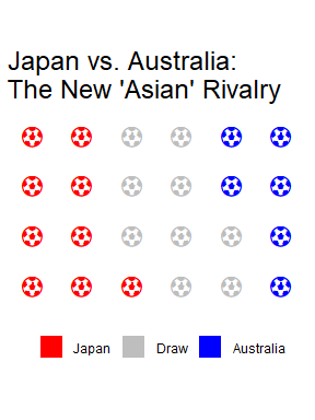
A new rival, Australia, emerged to challenge Japan in Asia as they joined the AFC in 2006. From the come-from-behind defeat in the Group Stages of the 2006 World Cup (still one of my most painful memories as a Japanese football fan…) and to an extra-time win in the 2011 Asian Cup Final (from a Zidane-esque finish by Tadanari Lee), Japan and Australia have dramatically clashed throughout the past decade.
Using the waffle package I can create a graphic that summarizes the
results between the two sides.
jp_aus <- results_jp_asia %>%
  japan_versus(opponent == "Australia") %>%
  select(-opponent, Japan = Win, Australia = Loss) %>%
  gather(key = "team", value = "values", -`Goals For`, -`Goals Against`) %>%
  select(-contains("Goals"))

# Waffle plot!
waffle(
  jp_aus, rows = 4, size = 1,
  title = glue("
               Japan vs. Australia:
               The New 'Asian' Rivalry"),
  colors = c("red", "grey", "blue"),
  use_glyph = "futbol", glyph_size = 5,
  legend_pos = "bottom"
)
Now let’s take a look at how Japan have historically played against the other teams in Group F of this year’s Asian Cup (in all competitions).
results_jp_asia %>%
  japan_versus(opponent %in% c("Oman", "Uzbekistan", "Turkmenistan")) %>%
  knitr::kable(format = "html",
               caption = "Japan's Record vs. Group F Teams") %>%
  kableExtra::kable_styling(full_width = FALSE) %>%
  kableExtra::add_header_above(c(" ", "Result" = 3, "Goals" = 2))
| opponent | Win | Draw | Loss | Goals For | Goals Against |
|---|---|---|---|---|---|
| Oman | 8 | 3 | 0 | 19 | 4 |
| Uzbekistan | 6 | 3 | 1 | 28 | 9 |
We see no rows here for Turkmenistan. This is due to the fact that until just this past week Japan had never played against them in a friendly or competitive game!
Conclusion
In this blog post I went through a few examples of visualizing some very basic stats on the Asian Cup happening this month. I’ll devote this last section on my views on this edition of the Asian Cup and Japan’s national team.
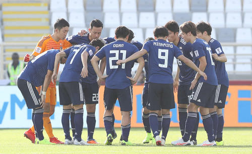
Although Japan’s first game was quite horrible I’m hoping it’ll wake the players and coaches out of their complacency and not underestimate our opponents in the next two games. Thankfully, South Korea should be on the other side of the bracket for the knock-out stages and we would also only meet Iran in the semifinals (provided both teams finish top of their respective groups). Japan could meet Australia in the Quarters but without Aaron Mooy they’re a much weaker side as shown in their abject loss to Jordan in their opening match.
Even with losing our new star, Shoya Nakajima, to injury the fact that we can replace him with a player of the calibre of Takashi Inui and with Hannover regular, Genki Haraguchi, stepping up from the bench shows how much Japanese football has progressed these past 25 years.
It’s a changing of the guard for Japan after the retirement of captain Hasebe and Keisuke Honda but with more Japanese players headed to Europe from a young age these are exciting times to be a Japanese football fan. It’s been quite awe-inspiring seeing how the number of Japanese players playing for foreign clubs have been steadily increasing since the 1988 Asian Cup squad (Japan’s first appearance at a major tournament, minus the Olympics).
This tournament is the first hurdle for this new generation of players as they fight to become regulars for the national team and begin the journey to the next World Cup in 2022. Here’s hoping for another great month of football!
(Image Source: Nikkan Sports)