Fans of soccer/football have been left bereft of their prime form of entertainment these past few months and I’ve seen a huge uptick in the amount of casual fans and bloggers turning to learning programming languages such as R or Python to augment their analytical toolkits. Free and easily accessible data can be hard to find if you only just started down this path and even when you do, you’ll find that eventually dragging your mouse around and copying stuff into Excel just isn’t time efficient or possible. The solution to this is web scraping! However, I feel like a lot of people aren’t aware of the ethical conundrums surrounding web scraping (especially if you’re coming from outside of a data science/programming/etc. background …and even if you are I might add). I am by no means an expert but since I started learning about it all I’ve tried to “web scrape responsibly” and this tenet will be emphasized throughout this blog post. I will be going over examples to scrape soccer data from Wikipedia, soccerway.com, and transfermarkt.com. Do note this is focused on the web-scraping part and won’t cover the visualization, links to the viz code will be given at the end of each section and you can always check out my soccer_ggplot Github repo for more soccer viz goodness!

Anyway, let’s get started!

Web Scraping Responsibly

When we think about R and web scraping, we normally just think straight to loading {rvest} and going right on our merry way. However, there are quite a lot of things you should know about web scraping practices before you start diving in. “Just because you can, doesn’t mean you should.” robots.txt is a file in websites that describe the permissions/access privileges for any bots and crawlers that come across the site. Certain parts of the website may not be accessible for certain bots (say Twitter or Google), some may not be available at all, and in the most extreme case, web scraping may even be prohibited. However, do note that just because there is no robots.txt file or that it is permissive of web scraping does not automatically mean you are allowed to scrape. You should always check the website’s “Terms of Use” or similar pages.

Web scraping takes up bandwidth for a host, especially if it houses lots of data. So writing web scraping bots and functions that are polite and respectful of the hosting site is necessary so that we don’t inconvenience websites that are doing us a service by making the data available for us for free! There’s a lot of things we take for granted, especially regarding free soccer data, so let’s make sure we can keep it that way.

In R there are a number of different packages that facilitates responsible web scraping packages, including:

• {robotstxt} is a package created by Peter Meissner and provides functions to parse robots.txt files in a clean way.

• {ratelimitr} created by Tarak Shah provides ways to limit the rate which functions are called. You can define a certain n calls per period of time to any function wrapped in ratelimitr::limit_rate().

The {polite} package takes a lot of the things previously mentioned into one neat package that flows seamlessly with the {rvest} API. I’ve been using this package almost since its first release and it’s terrific! I got to see the package author (Dmytro Perepolkin) do a presentation on it at UseR 2019 you can find the video recording here. This blog post will mainly focus on using {rvest} in combination with the {polite} package.

Single web-page (Wikipedia)

## On R 3.5.3
library(rvest)   # 0.3.5
library(polite)  # 0.1.1
library(dplyr)   # 0.8.5
library(tidyr)   # 1.0.2
library(purrr)   # 0.3.4
library(stringr) # 1.4.0
library(glue)    # 1.4.0
library(rlang)   # 0.4.6

For the first example, let’s start with scraping soccer data from Wikipedia, specifically the top goal scorers of the Asian Cup.

We use polite::bow() to pass the URL for the Wikipedia article to get a polite session object. This object will tell you about the robots.txt, the recommended crawl delay between scraping attempts, and tells you whether you are allowed to scrape this URL or not. You can also add your own user name in the user_agent argument to introduce yourself to the website.

topg_url <- "https://en.wikipedia.org/wiki/AFC_Asian_Cup_records_and_statistics"

session <- bow(topg_url,
               user_agent = "Ryo's R Webscraping Tutorial")

session

## <polite session> https://en.wikipedia.org/wiki/AFC_Asian_Cup_records_and_statistics
##     User-agent: Ryo's R Webscraping Tutorial
##     robots.txt: 454 rules are defined for 33 bots
##    Crawl delay: 5 sec
##   The path is scrapable for this user-agent

Of course, just to make sure, remember to read the “Terms of Use” page as well. When it comes to Wikipedia though, you could just download all of Wikipedia’s data yourself and do a text-search through those files but that’s out-of-scope for this blog post, maybe another time!

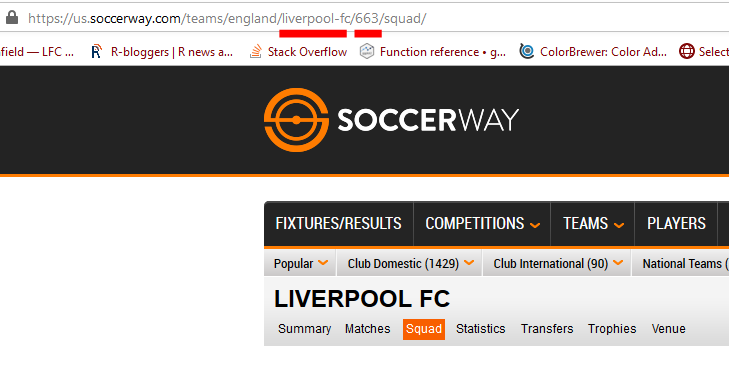
Now to actually get the data from the webpage. You’ve got different options depending on what browser you’re using but on Google Chrome or Mozilla Firefox you can find the exact HTML element by right clicking on it and then clicking on “Inspect” or “Inspect Element” in the pop-up menu. By doing so, a new view will open up showing you the full HTML content of the webpage with the element you chose highlighted. (See first two pics)

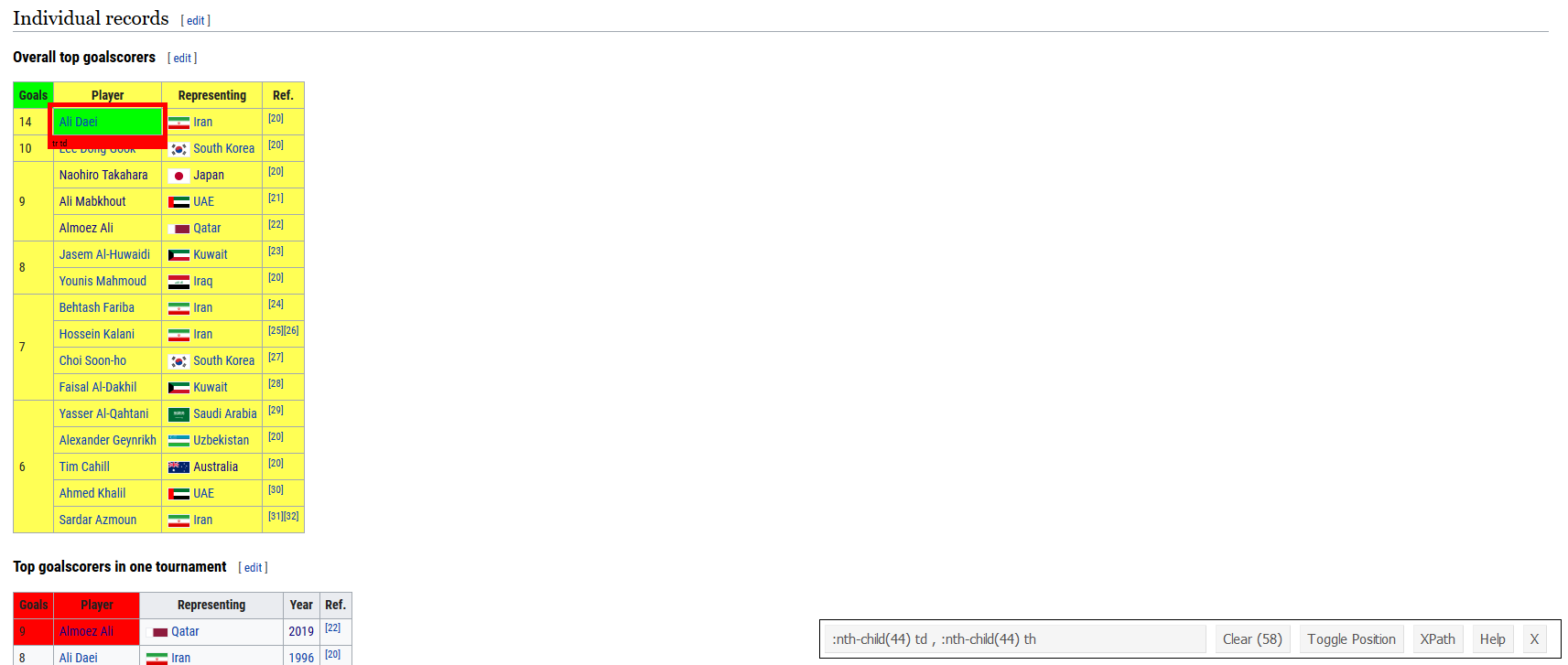
You might also want to try using a handy JavaScript tool called SelectorGadget, you can learn how to use it here. It allows you to click on different elements of the web page and the gadget will try to ascertain the exact CSS Selector in the HTML. (See bottom pic)

Do be warned that web pages can change suddenly and the CSS Selector you used in the past might not work anymore. I’ve had this happen more than a few times as pages get updated with more info from new tournaments and such. This is why you really should try to scrape from a more stable website, but a lot of times for “simple” data Wikipedia is the easiest and best place to scrape.

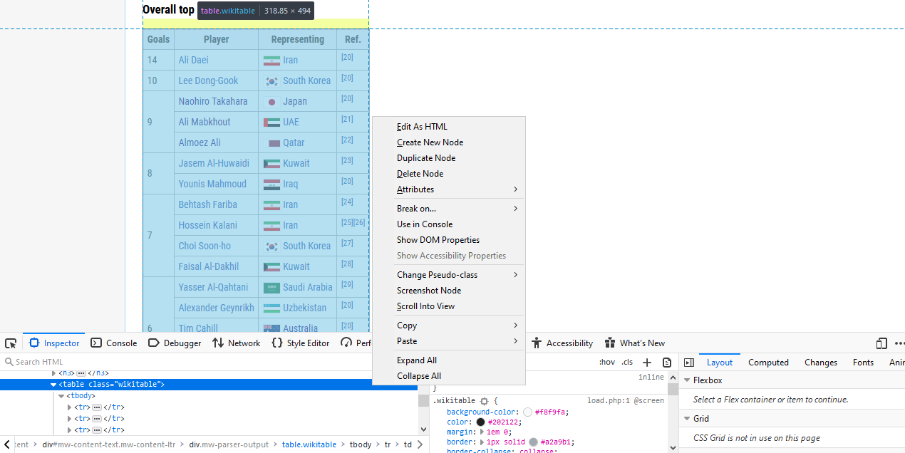
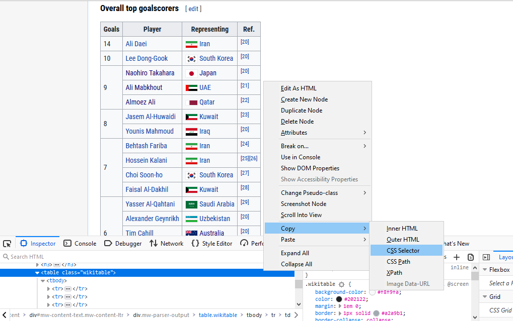
From here you can right-click again on the highlighted HTML code to “Copy”, and then you can choose one of “CSS Selector”, “CSS Path”, or “XPath”. I normally use “CSS Selector” and it will be the one I will use throughout this tutorial. This is the exact reference within the HTML code of the webpage of the object you want. I make sure to choose the CSS Selector for the table itself and not just the info inside the table.

With this copied, you can go to your R script/RMD/etc. After running the polite::scrape() function on your bow object, paste in the CSS Selector/Path/XPath you just copied into html_nodes(). The bow object already has the recommended scrape delay as stipulated in a website’s robots.txt so you don’t have to input it manually when you scrape.

ac_top_scorers_node <- scrape(session) %>%
  html_nodes("table.wikitable:nth-child(44)")

Grabbing a HTML table is the easiest way to get data as you usually don’t have to do too much work to reshape the data afterwards. We can do that with the html_table() function. As the HTML object returns as a list, we have to flatten it out one level using purrr::flatten_df() . Finish cleaning it up by taking out the unnecessary “Ref” column with select() and renaming the column names with set_names().

ac_top_scorers <- ac_top_scorers_node %>% 
  html_table() %>% 
  flatten_df() %>% 
  select(-Ref.) %>% 
  set_names(c("total_goals", "player", "country"))

After adding some flag and soccer ball images to the data.frame we get this:

Do note that the image itself is from before the 2019 Asian Cup but the data we scraped in the code above is updated. As a visualization challenge try to create a similar viz with the updated data! You can take a look at my Asian Cup 2019 blog post for how I did it. Alternatively you can try doing the same as above except with the Euros. Try grabbing the top goal scorer table from that page and make your own graph!

Single-page (Transfermarkt)

So now let’s try a soccer-specific website as that’s really the goal of this blog post. This time we’ll go for one of the most famous soccer websites around, transfermarkt.com. A website used as a data source from your humble footy blogger to big news sites such as the Financial Times and the BBC.

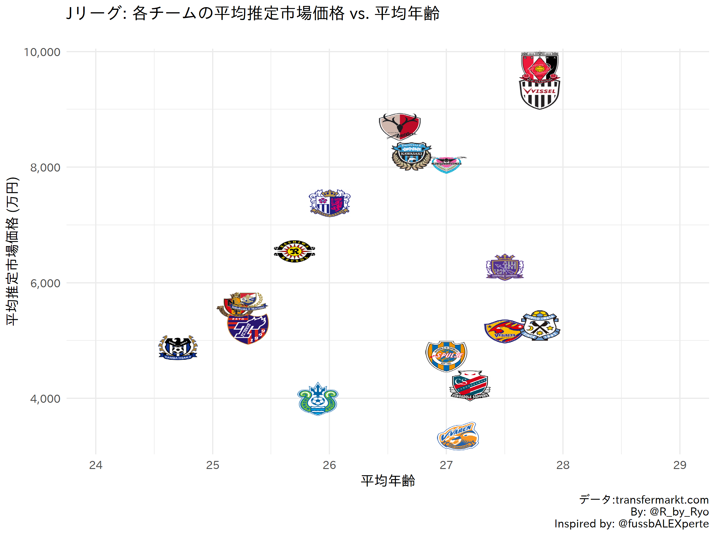
The example we’ll try is from an Age-Value graph for the J-League I made around 2 years ago when I just started doing soccer data viz (how times flies…).

url <- "https://www.transfermarkt.com/j-league-division-1/startseite/wettbewerb/JAP1/saison_id/2017"

session <- bow(url)

session

## <polite session> https://www.transfermarkt.com/j-league-division-1/startseite/wettbewerb/JAP1/saison_id/2017
##     User-agent: polite R package - https://github.com/dmi3kno/polite
##     robots.txt: 1 rules are defined for 1 bots
##    Crawl delay: 5 sec
##   The path is scrapable for this user-agent

• Terms of Use (in German)

The basic steps are the same as before but I’ve found that it can be quite tricky to find the right nodes on transfermarkt even with the CSS Selector Gadget or other methods we described in previous sections. After a while you’ll get used to the quirks of how the website is structured and know what certain assets (tables, columns, images) are called easily. This is a website where the SelectorGadget really comes in handy!

This time around I won’t be grabbing an entire table like I did with Wikipedia but a number of elements from the webpage. You definitely can scrape for the table like I showed above with html_table() but in this case I didn’t because the table output was rather messy, gave me way more info than I actually needed, and I wasn’t very good at regex/stringr to clean the text 2 years ago. Try doing it the way below and also by grabbing the entire table for more practice.

The way I did it back then also works out for this blog post because I can show you a few other html_*() {rvest} functions:

• html_table(): Get data from a HTML table
• html_text(): Extract text from HTML
• html_attr(): Extract attributes from HTML ("src" for image filename, "href" for URL link address)

team_name <- scrape(session) %>% 
  html_nodes("#yw1 > table > tbody > tr > td.zentriert.no-border-rechts > a > img") %>% 
  html_attr("alt")

# average age
avg_age <- scrape(session) %>% 
  html_nodes("tbody .hide-for-pad:nth-child(5)") %>% 
  html_text()

# average value
avg_value <- scrape(session) %>% 
  html_nodes("tbody .rechts+ .hide-for-pad") %>% 
  html_text()

# team image
team_img <- scrape(session) %>% 
  html_nodes("#yw1 > table > tbody > tr > td.zentriert.no-border-rechts > a > img") %>% 
  html_attr("src")

With each element collected we can put them into a list and reshape it into a nice data frame.

# combine above into one list
resultados <- list(team_name, avg_age, avg_value, team_img)

# specify column names
col_name <- c("team", "avg_age", "avg_value", "img")

# Combine into one dataframe
j_league_age_value_raw <- resultados %>% 
  reduce(cbind) %>% 
  tibble::as_tibble() %>% 
  set_names(col_name)

glimpse(j_league_age_value_raw)

## Rows: 18
## Columns: 4
## $ team      <chr> "Vissel Kobe", "Urawa Red Diamonds", "Kawasaki Frontale",...
## $ avg_age   <chr> "25.9", "26.3", "25.5", "24.1", "25.4", "25.0", "25.0", "...
## $ avg_value <chr> "€1.02m", "€698Th.", "€577Th.", "€477Th.", "€524Th.", "€5...
## $ img       <chr> "https://tmssl.akamaized.net/images/wappen/tiny/3958.png?...

With some more cleaning and {ggplot2} magic (see here, start from line 53) you will then get:

Some other examples by scraping single web pages:

• transfermarkt: simple age-utility plot from 2018
• “Winners of the Copa America” section of Visualizing the Copa America with R

Multiple Web-pages (Soccerway, Transfermarkt, etc.)

The previous examples looked at scraping from a single web page but usually you want to collect data for each team in a league, each player from each team, or each player from each team in every league, etc. This is where the added complexity of web-scraping multiple pages comes in. The most efficient way is to be able to programatically scrape across multiple pages in one go instead of running the same scraping function on different teams’/players’ URL link over and over again.

• Understand the website structure: How it organizes its pages, check out what the CSS Selector/XPaths are like, etc.
• Get a list of links: Team page links from league page, player page links from team page, etc.
• Create your own R functions: Pinpoint exactly what you want to scrape as well as some cleaning steps post-scraping in one function or multiple functions.
• Start small, then scale up: Test your scraping function on one player/team, then do entire team/league.
• Iterate over a set of URL links: Use {purrr}, for loops, lapply() (whatever your preference).

Look at the URL link for each web page you want to gather. What are the similarities? What are the differences? If it’s a proper website than the web page for a certain data view for each team should be exactly the same, as you’d expect it to contain exactly the same type of info just for a different team. For this example each “squad view” page for each Premier League team on soccerway.com are structured similarly: “https://us.soccerway.com/teams/england/” and then the “team name/”, the “team number/” and finally the name of the web page, “squad/”. So what we need to do here is to find out the “team name” and “team number” for each of the teams and store them. We can then feed each pair of these values in one at a time to scrape the information for each team.

url <- "https://us.soccerway.com/national/england/premier-league/20182019/regular-season/r48730/"

session <- bow(url)

session

## <polite session> https://us.soccerway.com/national/england/premier-league/20182019/regular-season/r48730/
##     User-agent: polite R package - https://github.com/dmi3kno/polite
##     robots.txt: 4 rules are defined for 3 bots
##    Crawl delay: 5 sec
##   The path is scrapable for this user-agent

• Terms of Use

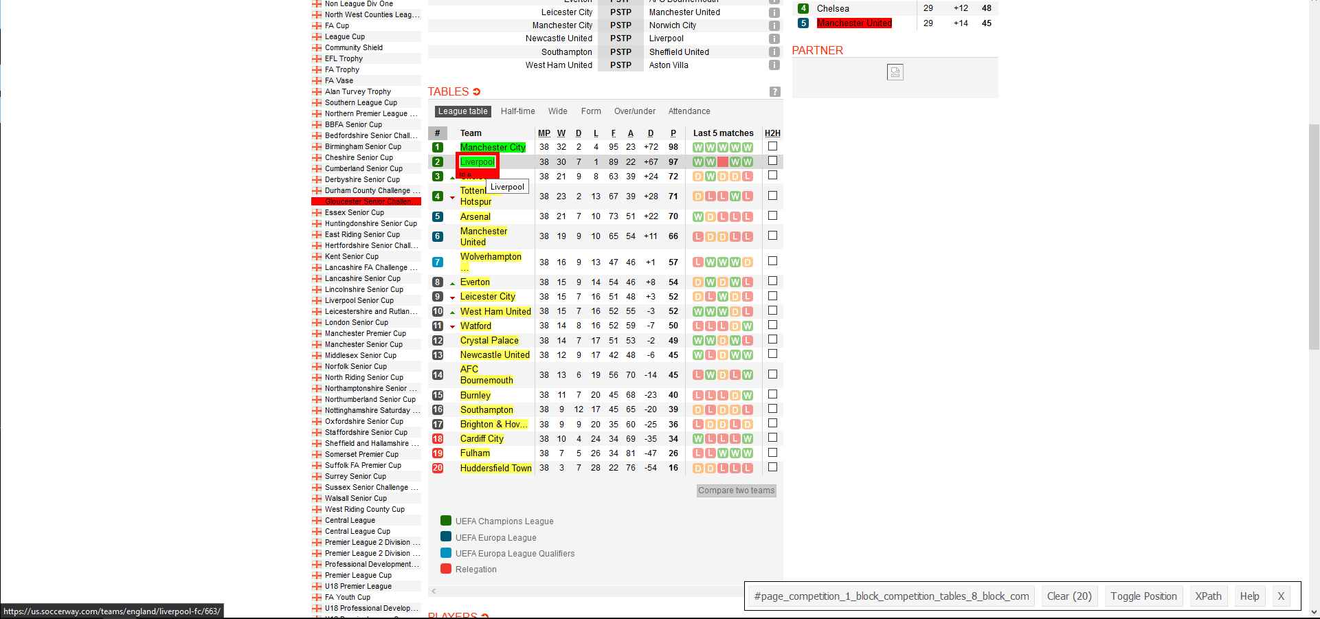
To find these elements we could just click on the link for each team and jot them down … but wait we can just scrape those too! We use the html_attr() function to grab the “href” part of the HTML, which contains the hyperlink of that element. The left picture is looking at the URL link of one of the buttons to a team’s page via “Inspect”. The right picture is selecting every team’s link via the SelectorGadget.

team_links <- scrape(session) %>% 
  html_nodes("#page_competition_1_block_competition_tables_8_block_competition_league_table_1_table .large-link a") %>% 
  html_attr("href")

team_links[[1]]

## [1] "/teams/england/manchester-city-football-club/676/"

The URL given in the href of the HTML for the team buttons unfortunately aren’t the full URL needed to access these pages. So we have to cut out the important bits and re-create them ourselves. We can use the {glue} package to combine the “team_name” and “team_num” for each team in the incomplete URL into a complete URL in a new column we’ll call link.

team_links_df <- team_links %>% 
  tibble::enframe(name = NULL) %>% 
  ## separate out each component of the URL by / and give them a name
  tidyr::separate(value, c(NA, NA, NA, "team_name", "team_num"), sep = "/") %>% 
  ## glue together the "team_name" and "team_num" into a complete URL
  mutate(link = glue("https://us.soccerway.com/teams/england/{team_name}/{team_num}/squad/"))

glimpse(team_links_df)

## Rows: 20
## Columns: 3
## $ team_name <chr> "manchester-city-football-club", "liverpool-fc", "chelsea...
## $ team_num  <chr> "676", "663", "661", "675", "660", "662", "680", "674", "...
## $ link      <glue> "https://us.soccerway.com/teams/england/manchester-city-...

Fantastic! Now we have the proper URL links for each team. Next we have to actually look into one of the web pages itself to figure out what exactly we need to scrape from the web page. This assumes that each web page and the CSS Selector for the various elements we want to grab are the same for every team. As this is for a very simple goal contribution plot all we need to gather from each team’s page is the “player name”, “number of goals”, and “number of assists”. Use the Inspect element or the SelectorGadget tool to grab the HTML code for those stats.

Below, I’ve split each into its own mini-scraper function. When you’re working on this part, you should try to use the URL link from one team and build your scraper functions from that link (I usually use Liverpool as my test example when scraping Premier League teams). Note that all three of the mini-functions below could just be chucked into one large function but I like keeping things compartmentalized.

player_name_info <- function(session) {
  
  player_name_info <- scrape(session) %>% 
    html_nodes("#page_team_1_block_team_squad_3-table .name.large-link") %>% 
    html_text()
}

num_goals_info <- function(session) {

  num_goals_info <- scrape(session) %>% 
    html_nodes(".goals") %>% 
    html_text()
  
  ## first value is blank so remove it
  num_goals_info_clean <- num_goals_info[-1]
}

num_assists_info <- function(session) {

  num_assists_info <- scrape(session) %>% 
    html_nodes(".assists") %>% 
    html_text()
  
  ## first value is blank so remove it
  num_assists_info_clean <- num_assists_info[-1]
}

Now that we have scrapers for each stat, we can combine these into a larger function that will then gather them all up into a nice data frame for each team that we want to scrape. If you input any one of the team URLs from team_links_df, it will collect the “player name”, “number of goals”, and “number of assists” for that team.

premier_stats_info <- function(link, team_name) {
  
  team_name <- rlang::enquo(team_name)
  ## `bow()` for every URL link
  session <- bow(link)
  
  ## scrape different stats
  player_name <- player_name_info(session = session)

  num_goals <- num_goals_info(session = session)

  num_assists <- num_assists_info(session = session)
  
  ## combine stats into a data frame
  resultados <- list(player_name, num_goals, num_assists)
  col_names <- c("name", "goals", "assists") 
  
  premier_stats <- resultados %>% 
    reduce(cbind) %>% 
    as_tibble() %>% 
    set_names(col_names) %>% 
    mutate(team = !!team_name)
  
  ## A little message to keep track of how the function is progressing:
  # cat(team_name, " done!")
  
  return(premier_stats)
}

Iteration Over a Set of Links

OK, so now we have a function that can scrape the data for ONE team but it would be extremely ponderous to re-run it another NINETEEN times for all the other teams… so what can we do? This is where the purrr::map() family of functions and iteration comes in! The map() family of functions allows you to apply a function (an existing one from a package or one that you’ve created yourself) to each element of a list or vector that you pass as an argument to the mapping function. For our purposes, this means we can use mapping functions to pass along a list of URLs (for whatever number of players and/or teams) along with a scraping function so that it scrapes it altogether in one go.

In addition, we can use purrr::safely() to wrap any function (including custom made ones). This makes these functions return a list with the components result and error. This is extremely useful for debugging complicated functions as the function won’t just error out and give you nothing, but at least the result of the parts of the function that worked in result with what didn’t work in error.

So for example, say you are scraping data from the webpage of each team in the Premier League (by iterating a single scraping function over each teams’ web page) and by some weird quirk in the HTML of the web page or in your code, the data from one team errors out (while the other 19 teams’ data are gathered without problems). Normally, this will mean the data you gathered from all other web pages that did work won’t be returned, which can be extremely frustrating. With a safely() wrapped function, the data from the 19 teams’ data that the function was able to scrape is returned in result component of the list object while the one errored team and error message is returned in the error component. This makes it very easy to debug when you know exactly which iteration of the function failed.

safe_premier_stats_info <- safely(premier_stats_info)

We already have a nice list of team URL links in the data frame team_links_df, specifically in the “link” column (team_links_df$link). So we pass that along as an argument to map2() (which is just a version of map() but for two argument inputs) and our premier_stats_info() function so that the function will be applied to each team’s URL link. This part may take a while depending on your internet connection and/or if you put a large value for the crawl delay.

goal_contribution_df_ALL <- map2(.x = team_links_df$link, .y = team_links_df$team_name,
                             ~ safe_premier_stats_info(link = .x, team_name = .y))

## check out the first 4 results:
glimpse(head(goal_contribution_df_ALL, 4))

As you can see (the results/errors for the first four teams scraped), for each team there is a list holding a “result” and “error” element. For the first four, at least, it looks like everything was scraped properly into a nice data.frame. We can check if any of the twenty teams had an error by purrr::discard()-ing any elements of the list that come out as NULL and seeing if there’s anything left.

## check to see if any failed:
goal_contribution_df_ALL %>% 
  map("error") %>% 
  purrr::discard(~is.null(.))

## list()

It comes out as a empty list which means were no errors in the “error” elements. Now we can squish and combine individual team data.frames into one data.frame using dplyr::bind_rows().

goal_contribution_df <- goal_contribution_df_ALL %>% 
  map("result") %>% 
  bind_rows()

glimpse(goal_contribution_df)

## Rows: 622
## Columns: 4
## $ name    <chr> "C. Bravo", "Ederson Moraes", "S. Carson", "K. Walker", "J....
## $ goals   <chr> "0", "0", "0", "1", "0", "0", "0", "0", "0", "2", "0", "0",...
## $ assists <chr> "0", "0", "0", "2", "0", "0", "0", "2", "0", "0", "0", "0",...
## $ team    <chr> "manchester-city-football-club", "manchester-city-football-...

With that we can clean the data a bit and finally get on to the plotting! You can find the code in the original gist to see how I created the plot below. I really would like to go into detail especially as I use one of my favorite plotting packages, {ggforce}, here but it deserves its own separate blog post. NOTE: The data we scraped in the above section is for this season (2019-2020) so the annotations won’t be the same as in the original gist which is for 2018-2019. Try to play around with the different annotations options in R as practice!

As you can see, this one was for the 2018-2019 season. I made a similar one but using xG per 90 and xA per 90 for the 2019-2020 season (as per January 1st, 2020 at least) using FBRef data here. You can find the code for it here. However, I did not web scrape it as from their Terms of Use page, FBRef (or any of the SportsRef websites) do not allow web scraping (“spidering”, “robots”). Thankfully, they make it very easy to access their data as downloadable .csv files by just clicking on a few buttons, so getting their data isn’t really a problem!

For practice, try doing it for a different season or for a different league altogether!

For other examples of scraping multiple pages:

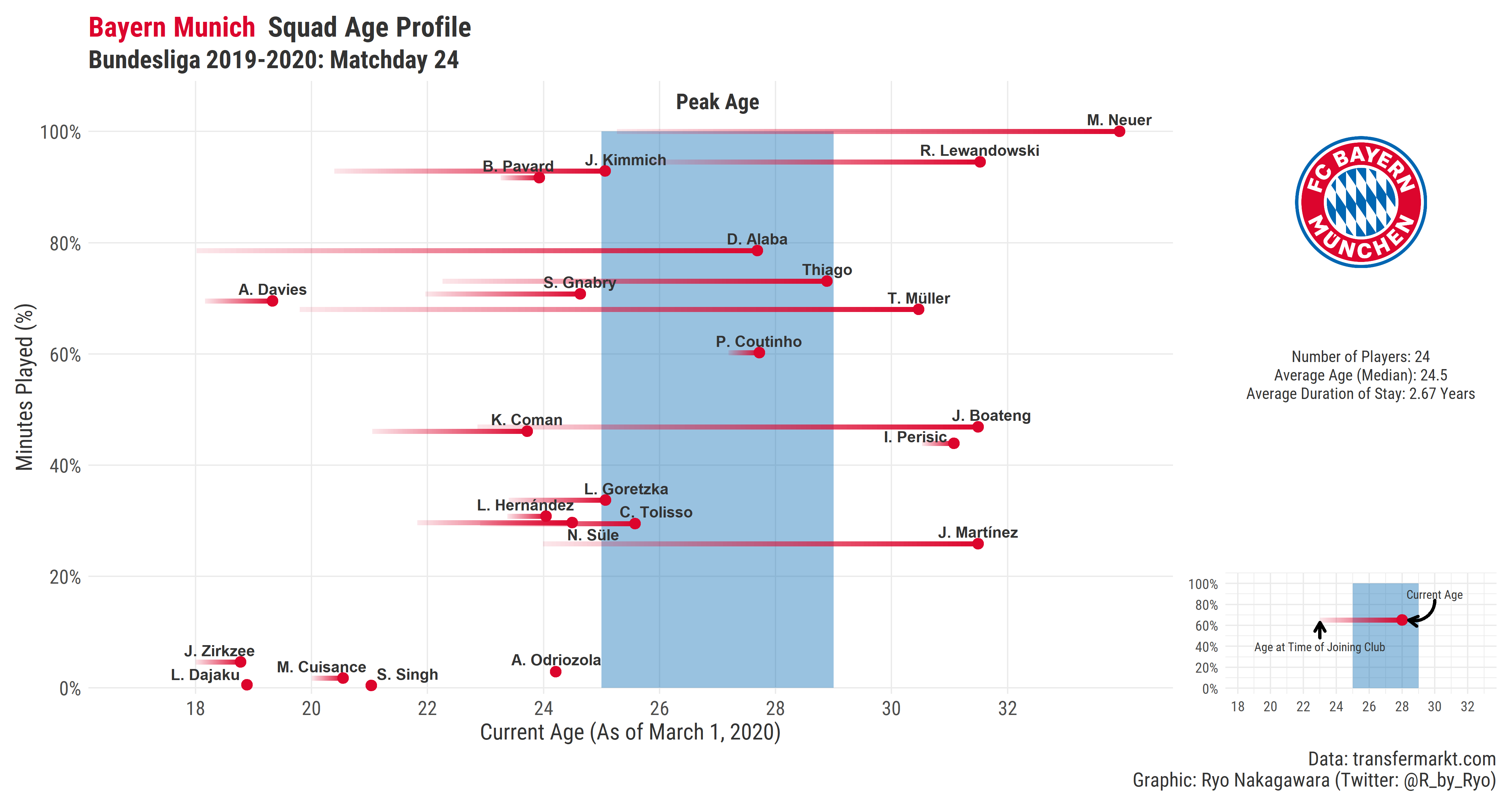
• transfermarkt: (Opta-inspired Age-Utility plot from February 28, 2020)
• Age-Utility plots for most major European teams (Twitter thread)

Conclusion

This blog post went over web-scraping, focusing on getting soccer data from soccer websites in a responsibly fashion. After a brief overview of responsible scraping practices with R I went over several examples of getting soccer data from various websites. I make no claims that its the most efficient way, but importantly, it gets the job done and in a polite way. More industrial-scale scraping over hundreds and thousands of web pages is a bit out of scope for an introductory blog post and it’s not something I’ve really done either, so I will pass along the torch to someone else who wants to write about that. There are other ways to scrape websites using R, especially websites that have dynamic web pages, using R Selenium, Headless Chrome (crrri), and other tools.

In regards to FBRef, as it is now a really popular website to use (especially with their partnership with StatsBomb), there is a blog post out there detailing a way of using R Selenium to get around the terms stipulated and the reasoning seems OK but I am still not 100% sure. This goes again into how a lot of web scraping can be in a rather grey area at times, as for all the clear warnings on some websites you have a lot more ambiguity and ability to use some expedient interpretation in others. At the end of the day, you just have to do your due diligence, ask permission directly if possible, and be {polite} about it.

Some other web-scraping tutorials you might be interested in:

• Harvesting the web with rvest (rvest package vignette)
• Web scraping the {polite} way

As always, you can find more of my soccer-related stuff on this website or on soccer_ggplots Github repo!

Happy (responsible) Web-scraping!